
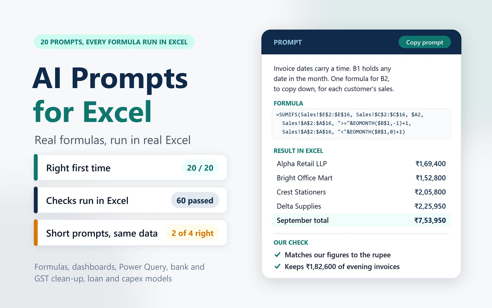
Most lists of AI prompts for Excel stop at the prompt. We ran twenty of them, pasted every formula the AI wrote into a real Excel workbook with the sample data, and checked what came out.
These AI prompts for Excel cover the work finance teams do in spreadsheets every week: SUMIFS and XLOOKUP formulas, financial-year dates, trial balance mapping, bank statement clean-up, duplicate bills, reconciliations, GSTIN checks, Power Query, ageing, dashboards, variance analysis, loan and capex models, and fixing a workbook that gives the wrong answer. Each card has the prompt with its sample data, the answer Claude Opus 5.5 gave, and what happened when we ran it.
How we tested
- Model: Claude Opus 5.5, in a fresh session for every prompt, with no files, memory or web search. It saw only the prompt you can copy below.
- Data: the same fictional distributor as our AI prompts for accounting, Acme Traders Private Limited in Pune. We planted the traps real files have: invoice times on the last day of the month, codes stored as text, a Saturday working week, a party name with a slash in it, two payments of the same amount on the same day, and a bank file opened on a laptop set to US dates.
- Excel check: we ran every formula, the Power Query and the LAMBDA in Excel for Microsoft 365 on Windows, in a fresh workbook with the prompt’s data, and compared each result with figures we had worked out separately. Prompts written for Excel 2019 were entered the way Excel 2019 evaluates them.
- Date: 27 September 2026.
AI prompts for Excel: the scorecard
All 20 of the 20 AI prompts for Excel came back right first time. That is 60 separate checks in Excel, and not one failed. Every planted trap was caught, and in two answers the AI found a problem we had not planted. The reason is in the prompts as much as the model: each one names the Excel version, says where the data sits and states the rule. The side test further down shows what happens when a prompt leaves those out.
| # | Prompt | Result in Excel | What to watch |
|---|---|---|---|
| 1 | Monthly sales by customer with SUMIFS | Right | Nothing; right first time |
| 2 | New-regime income tax with rebate and marginal relief | Right | Nothing; add a band if anyone earns over ₹1 crore |
| 3 | Financial year, quarter and due-date formulas | Right | Nothing; add next year’s holidays |
| 4 | Map a trial balance to Schedule III heads | Right | Nothing; add a range for capital work-in-progress |
| 5 | Unique vendor list with totals in Excel 2019 | Right | Nothing; right first time |
| 6 | Amount in words in Indian format, without macros | Right | Nothing; needs Excel 2024 or Microsoft 365 |
| 7 | Fix dates and amounts from a bank CSV | Right | Nothing; only for files opened by double-click |
| 8 | Split UPI and NEFT narrations into columns | Right | Nothing; watch remarks that contain a slash |
| 9 | Find duplicate vendor invoices | Right | Nothing; hold flagged bills, do not auto-reject |
| 10 | Match book payments to the bank one to one | Right | Nothing; keep Books in date order |
| 11 | Validate GSTINs, including the check digit | Right | Nothing; confirm new vendors on the GST portal |
| 12 | Power Query to import a bank CSV | Right | Nothing; do not add an auto type step later |
| 13 | Receivables ageing with buckets and a summary | Right | Nothing; right first time |
| 14 | Plan a sales dashboard and its KPI formulas | Right | Nothing; check Delta’s order before the pack goes out |
| 15 | Budget vs actual variance analysis with commentary | Right | Nothing; right first time |
| 16 | Loan EMI schedule with a prepayment | Right | Nothing; the bank may round differently |
| 17 | NPV, IRR and payback for a capex proposal | Right | Nothing; confirm the savings are after tax |
| 18 | Fix a wrong total and a wrong lookup | Right | Nothing; it found more than we asked |
| 19 | Explain and simplify an inherited formula | Right | Nothing; right first time |
| 20 | Review a budget model for errors | Right | Nothing; right first time |
How to write AI prompts for Excel formulas
Every prompt on this page has the same six parts. Keep them and you can write your own AI prompts for Excel formulas for any task.
- Your Excel version. “Excel 2019”, “Excel 2021” or “Microsoft 365”. It decides whether you get XLOOKUP, LAMBDA or an older INDEX and MATCH formula that works on your machine.
- The layout. The sheet name, the range, the header row, and whether each column holds text, numbers, dates or dates with times.
- A few rows of data. Paste them as a table. Include the awkward rows: the credit note, the blank line, the code with a leading zero.
- The rule in your words. Your working week, your ageing buckets, your definition of a duplicate. The AI cannot know your office’s rules.
- The output. “One formula for row 2 to copy down”, “one formula that spills”, or “the complete M code”.
- The results to expect. Ask the AI to show what the formula should return for your rows. You can then check it in a minute instead of trusting it.
For the formulas themselves, with worked finance examples, see our guide to Excel formulas for finance.
AI prompts for Excel formulas
These AI prompts for Excel formulas cover the lookups, date logic and calculations finance teams write every week. Each one says which Excel you use, where the data sits and what the result should be, which is what lets the AI write a formula you can paste straight in.
1. Monthly sales by customer with SUMIFS
Use it for: monthly totals by customer, vendor or ledger from a register whose dates carry a time.
I am the accountant of Acme Traders Private Limited, a distributor of office supplies in Pune, Maharashtra. We use Excel for Microsoft 365.

The sheet Sales holds our invoice register in A1:E16, with headers in row 1:
- Column A: invoice date and time, as real Excel date-time values exported from our billing system.
- Column B: invoice or credit note number.
- Column C: customer.
- Column D: state.
- Column E: taxable value in rupees. Credit notes are negative.

On a sheet named Summary, A2:A5 list our four customers and B1 holds a date in the month we want to report. We type any date in that month, for example 15-09-2026.

Write:
1. One formula for Summary!B2, to copy down to B5, that returns each customer's taxable value for the month in B1.
2. A formula for B6 that returns the month's total for all customers.
3. A formula for B7 that shows OK if B6 equals the total of B2:B5, and Check if it does not.

Explain each formula in one or two lines, then show the results you expect for September 2026 from this data.

| Invoice date and time | Number | Customer | State | Taxable value (₹) |
|---|---|---|---|---|
| 28-08-2026 11:20 | AT/0981 | Alpha Retail LLP | Maharashtra | 84,000 |
| 31-08-2026 23:10 | AT/0990 | Bright Office Mart | Gujarat | 56,500 |
| 01-09-2026 09:05 | AT/0991 | Alpha Retail LLP | Maharashtra | 1,18,000 |
| 04-09-2026 15:40 | AT/0996 | Crest Stationers | Karnataka | 42,300 |
| 09-09-2026 12:00 | AT/1004 | Delta Supplies | Maharashtra | 76,250 |
| 12-09-2026 17:30 | AT/1011 | Bright Office Mart | Gujarat | 1,05,000 |
| 15-09-2026 10:15 | AT/1019 | Alpha Retail LLP | Maharashtra | 63,400 |
| 18-09-2026 16:50 | AT/1026 | Crest Stationers | Karnataka | 38,900 |
| 22-09-2026 11:45 | AT/1033 | Delta Supplies | Maharashtra | 91,700 |
| 25-09-2026 14:20 | CN/0042 | Alpha Retail LLP | Maharashtra | -12,000 |
| 27-09-2026 13:05 | AT/1043 | Bright Office Mart | Gujarat | 47,800 |
| 30-09-2026 18:45 | AT/1049 | Crest Stationers | Karnataka | 1,24,600 |
| 30-09-2026 21:30 | AT/1050 | Delta Supplies | Maharashtra | 58,000 |
| 01-10-2026 10:10 | AT/1051 | Alpha Retail LLP | Maharashtra | 72,000 |
| 02-10-2026 12:30 | AT/1054 | Crest Stationers | Karnataka | 49,900 |

Summary!A2:A5 hold: Alpha Retail LLP, Bright Office Mart, Crest Stationers, Delta Supplies.
=SUMIFS(Sales!$E$2:$E$16, Sales!$C$2:$C$16, $A2, Sales!$A$2:$A$16, ">="&EOMONTH($B$1,-1)+1, Sales!$A$2:$A$16, "<"&EOMONTH($B$1,0)+1)
[…] Ending at “before next month starts” rather than “up to the last day” keeps evening invoices on the 30th. […]
"<="&EOMONTH($B$1,0)stops at 30-09-2026 00:00 and drops AT/1049 (18:45) and AT/1050 (21:30). Crest would fall to 81,200, Delta to 1,67,950 and the total to 5,71,350.
B7 would still show OK in both cases, because B6 uses the same window as B2:B5.
- ✓ In Excel the formulas returned exactly our totals: ₹1,69,400, ₹1,52,800, ₹2,05,800 and ₹2,25,950, a month total of ₹7,53,950, and OK.
- ✓ It caught both traps: the date typed in B1 is mid-month, and two invoices on 30 September carry evening times. We ran the version it warned against: Crest drops to ₹81,200, just as it said.
- ✓ It pointed out something we had not asked: the OK check cannot catch a wrong date window, because both sides use the same window.
Prompt tip: Say that the dates carry a time and that the month cell may hold any date in the month. Those two lines are what make the formula robust.
2. New-regime income tax with rebate and marginal relief
Use it for: a payroll tax estimate for tax year 2026-27 under the new regime, with the rates kept in a table.
I am the payroll accountant of Acme Traders Private Limited, a distributor of office supplies in Pune, Maharashtra. We use Excel for Microsoft 365. I need formulas to estimate each employee's income tax for tax year 2026-27 under the new regime (the default regime).

Sheet Tax: A2:A9 hold employee codes and B2:B9 the gross salary for the year in rupees. All are resident individuals below 60 with salary income only and no other deductions.

Rules to apply:
- Standard deduction: ₹75,000.
- Slabs on taxable income: up to ₹4,00,000 nil; ₹4,00,001 to ₹8,00,000 5%; ₹8,00,001 to ₹12,00,000 10%; ₹12,00,001 to ₹16,00,000 15%; ₹16,00,001 to ₹20,00,000 20%; ₹20,00,001 to ₹24,00,000 25%; above ₹24,00,000 30%.
- Rebate: up to ₹60,000 if taxable income does not exceed ₹12,00,000, with marginal relief for income just above ₹12,00,000.
- Surcharge: 10% of tax if taxable income exceeds ₹50,00,000, with marginal relief.
- Health and education cess: 4% of tax plus surcharge.

Write formulas for row 2, to copy down, for C (taxable income), D (tax on the slabs), E (tax after the rebate and marginal relief), F (surcharge after marginal relief), G (cess) and H (total tax, rounded to the nearest ₹10). Keep the slab table on the sheet instead of hard-coding the rates in the formula, and tell me where you put it. Then show the results you expect for these eight employees.

| Employee | Gross salary (₹) |
|---|---|
| E01 | 7,50,000 |
| E02 | 12,75,000 |
| E03 | 12,85,000 |
| E04 | 13,45,000 |
| E05 | 13,50,000 |
| E06 | 18,00,000 |
| E07 | 50,75,000 |
| E08 | 51,25,000 |
E2: Tax after rebate and marginal relief
=IF(C2<=$O$3,MAX(0,D2-$O$4),MIN(D2,C2-$O$3))
F2: Surcharge after marginal relief
=IF(C2<=$O$5,0,MIN(E2*$O$6,C2-$O$5-(E2-$O$8)))
| Employee | Taxable income (C) | Tax on slabs (D) | After rebate (E) | Surcharge (F) | Total tax (H) |
|---|---|---|---|---|---|
| E03 | 12,10,000 | 61,500 | 10,000 | 0 | 10,400 |
| E04 | 12,70,000 | 70,500 | 70,000 | 0 | 72,800 |
| E08 | 50,50,000 | 10,95,000 | 10,95,000 | 35,000 | 11,75,200 |
- ✓ All eight totals matched ours in Excel, from ₹0 at ₹12,75,000 of salary to ₹11,75,200 at ₹51,25,000.
- ✓ Both marginal reliefs are right: the rebate relief just above ₹12 lakh (sections 156 and 202 of the Income-tax Act, 2025) and the surcharge relief just above ₹50 lakh, which cuts ₹1,09,500 to ₹35,000.
- ✓ It flagged the limits of its own formula: incomes above ₹1 crore need the 15% surcharge band, and Excel 2019 users must enter two cells with Ctrl+Shift+Enter.
Prompt tip: Give the slabs, rebate and surcharge rules in the prompt, as here. The formula is only as current as the rates you give it; check them each Budget on our income tax slab rates page.
3. Financial year, quarter and due-date formulas
Use it for: financial year and quarter labels, GST due dates and MSME payment scheduling for an office that works six days a week.
I am the accountant of Acme Traders Private Limited, a distributor of office supplies in Pune, Maharashtra. We use Excel for Microsoft 365. Our office works Monday to Saturday; Sunday is the weekly off. We file GSTR-3B monthly.

Sheet Dates: A2:A9 hold supplier invoice dates (real dates) and H2:H8 hold our office holidays. Write formulas for row 2, to copy down, for:
B. the financial year of the invoice date, shown like 2026-27 (April to March),
C. the quarter of that financial year, shown as Q1 to Q4 (Q1 is April to June),
D. the GSTR-3B due date for the month of the invoice (the 20th of the next month),
E. the MSME payment deadline, 45 days after the invoice date (treat the invoice date as the day of acceptance),
F. the date to schedule the payment: the last working day on or before the deadline in E,
G. the number of working days from the invoice date to the date in F, counting both days.

Then show the results you expect for every row.

Invoice dates (A2:A9): 15-01-2026, 31-03-2026, 01-04-2026, 17-08-2026, 18-08-2026, 30-09-2026, 20-11-2026, 31-12-2026.
Office holidays (H2:H8): 26-01-2026, 15-08-2026, 02-10-2026, 20-10-2026, 09-11-2026, 25-12-2026, 01-01-2027.
| Cell | Formula |
|---|---|
| B2 | =LET(y, YEAR(A2)-(MONTH(A2)<4), y&"-"&RIGHT(y+1,2)) |
| C2 | ="Q"&CHOOSE(MONTH(A2),4,4,4,1,1,1,2,2,2,3,3,3) |
| F2 | =WORKDAY.INTL(E2+1,-1,11,$H$2:$H$8) |
| G2 | =NETWORKDAYS.INTL(A2,F2,11,$H$2:$H$8) |
[…] Under Section 15 of the MSMED Act, 45 days is the maximum credit period and applies only when it is agreed in writing; without a written agreement the limit is 15 days from acceptance […]
- ✓ Every date and count matched ours in Excel: financial years, quarters, all eight GSTR-3B due dates, payment dates and working days (38, 40, 40, 40, 39, 37, 37, 38).
- ✓ It used weekend code 11, so Saturdays stay working days. We ran plain WORKDAY as a control: it moved the Saturday deadline of 16 May 2026 back to Friday.
- ✓ It added two correct points we had not asked for: the 15-day limit without a written agreement, and the exclusion of traders and medium enterprises.
Prompt tip: State your working week. “Monday to Saturday” is the single line that changes the answer, as our short-prompt test below shows.
4. Map a trial balance to Schedule III heads
Use it for: mapping a trial balance to Schedule III heads when codes come out of the software as text.
I am the accountant of Acme Traders Private Limited, a distributor of office supplies in Pune, Maharashtra. We use Excel for Microsoft 365. I want to map our trial balance at 30 September 2026 to Schedule III heads.

Sheet TB (A1:C24, headers in row 1): A = GL code, B = GL name, C = closing balance in rupees (debit positive, credit negative). The GL codes came from our accounting software, so they are stored as text.

Sheet Map (A1:C16, headers in row 1): code ranges, with the From and To codes stored as numbers:

| From | To | Schedule III head |
|---|---|---|
| 10000 | 10999 | Share capital |
| 11000 | 11999 | Other equity |
| 20000 | 20999 | Borrowings |
| 21000 | 21999 | Trade payables |
| 22000 | 22999 | Other current liabilities |
| 30000 | 30999 | Property, plant and equipment |
| 32000 | 32999 | Inventories |
| 33000 | 33999 | Trade receivables |
| 34000 | 34999 | Cash and cash equivalents |
| 40000 | 40999 | Revenue from operations |
| 41000 | 41999 | Other income |
| 50000 | 50999 | Purchases of stock-in-trade |
| 51000 | 51999 | Employee benefits expense |
| 52000 | 52999 | Finance costs |
| 53000 | 53999 | Other expenses |

Sheet Exceptions (A1:B4, headers in row 1): single codes, stored as numbers, that override their range:

| Code | Schedule III head |
|---|---|
| 22150 | Borrowings |
| 34900 | Other bank balances |
| 53410 | Finance costs |

Write:
1. A formula for TB!D2, to copy down, that returns the Schedule III head: the exception if there is one, otherwise the range the code falls in, and Unmapped if the code is in no range.
2. On a sheet named Summary, A2:A18 list the 16 heads and Unmapped. A formula for B2, to copy down, that totals the balances for each head.
3. Two checks: the trial balance totals zero, and nothing is unmapped.

Then show the head you expect for each GL and the summary.

| GL code | GL name | Balance (₹) |
|---|---|---|
| 10100 | Equity share capital | -10,00,000 |
| 11200 | Retained earnings | -18,45,000 |
| 20100 | Term loan from bank | -6,40,000 |
| 21050 | Sundry creditors | -9,72,400 |
| 22150 | Current maturities of term loan | -2,40,000 |
| 22400 | GST payable | -1,86,300 |
| 30100 | Furniture and fixtures | 7,85,000 |
| 31500 | Capital work-in-progress | 3,20,000 |
| 32100 | Stock-in-trade | 14,60,000 |
| 33100 | Sundry debtors | 12,35,600 |
| 34100 | Cash on hand | 48,200 |
| 34200 | Current account | 6,92,100 |
| 34900 | Fixed deposit, 9 months | 5,00,000 |
| 40100 | Sales of office supplies | -62,40,000 |
| 41300 | Interest on fixed deposit | -41,200 |
| 50100 | Purchases | 44,35,000 |
| 51100 | Salaries and wages | 9,80,000 |
| 52100 | Interest on term loan | 78,500 |
| 53200 | Rent | 3,60,000 |
| 53410 | Interest on MSME dues | 12,300 |
| 53500 | Power and fuel | 1,05,500 |
| 53800 | Audit fees | 1,50,000 |
| 60100 | Suspense account | 2,700 |
=LET(
    gl,      VALUE(TRIM(A2)),
    byRange, XLOOKUP(1, (Map!$A$2:$A$16<=gl)*(Map!$B$2:$B$16>=gl), Map!$C$2:$C$16, "Unmapped"),
    head,    XLOOKUP(gl, Exceptions!$A$2:$A$4, Exceptions!$B$2:$B$4, byRange),
    IFERROR(head, "Unmapped")
)
[…] An approximate match (VLOOKUP with TRUE, or XLOOKUP match mode -1) reads only the From column, so it would quietly put 31500 into Property, plant and equipment and 60100 into Other expenses.
- ✓ In Excel, all 23 codes landed on the right head and the 17 summary totals matched ours, with ₹3,22,700 left Unmapped.
- ✓ It found both planted gaps: capital work-in-progress between two ranges and a suspense code above them all. It converted the text codes before comparing.
- ✓ It added two correct Schedule III points: capital work-in-progress is its own line with an ageing schedule, and “Other equity” is Ind AS (Division II) wording.
Prompt tip: Say which columns are text and which are numbers. Most broken lookups are a text 22150 meeting a number 22150.
5. Unique vendor list with totals in Excel 2019
Use it for: a unique list with totals on older Excel, where UNIQUE and FILTER do not exist.
I am the accountant of Acme Traders Private Limited, a distributor of office supplies in Pune, Maharashtra. Our office uses Excel 2019.

Sheet Purchases has our September 2026 purchase bills in A1:D16, with headers in row 1: A = bill date, B = vendor, C = bill number, D = amount in rupees. Row 9 is empty because a line was deleted.

I want, on the same sheet:
- F2 downwards: each vendor once, in the order they first appear.
- G2 downwards: the total amount for that vendor.
The formulas should show a blank once the list runs out, and should keep working when we add bills down to row 500.

Give me the formulas, tell me exactly how to enter them, and show the list and totals you expect.

| Row | Date | Vendor | Bill no | Amount (₹) |
|---|---|---|---|---|
| 2 | 02-09-2026 | Redline Couriers | RC/2026/118 | 9,800 |
| 3 | 03-09-2026 | Blue Pine Computers | BP-4471 | 99,120 |
| 4 | 05-09-2026 | Zen Properties | ZP/SEP/26 | 90,000 |
| 5 | 08-09-2026 | Kavya and Associates | 1001 | 45,000 |
| 6 | 10-09-2026 | Redline Couriers | RC/2026/124 | 7,450 |
| 7 | 12-09-2026 | Greenfield Security Services | GS 2231 | 50,000 |
| 8 | 15-09-2026 | Blue Pine Computers | BP-4490 | 18,880 |
| 9 | | | | |
| 10 | 18-09-2026 | Orbit Stationery | OS/778 | 23,450 |
| 11 | 20-09-2026 | Silverleaf Consultants | SC-1187 | 1,41,600 |
| 12 | 22-09-2026 | Redline Couriers | RC/2026/131 | 9,800 |
| 13 | 25-09-2026 | Orbit Stationery | OS/781 | 12,300 |
| 14 | 28-09-2026 | Zen Properties | ZP/SEP/26A | 4,500 |
| 15 | 29-09-2026 | Kavya and Associates | 1019 | 15,000 |
| 16 | 30-09-2026 | Greenfield Security Services | GS 2240 | 50,000 |
Excel 2019 does not have UNIQUE or FILTER. Those came with Microsoft 365 and Excel 2021. […]
F2: vendor list (array formula, entered with Ctrl+Shift+Enter)
=IFERROR(INDEX($B$2:$B$500,MATCH(0,COUNTIF($F$1:F1,$B$2:$B$500)+($B$2:$B$500=""),0)),"")
[…] Do not select F2:F101 and press Ctrl+Shift+Enter once. That creates one block formula, and every cell shows Redline Couriers.
- ✓ We entered the formula the way Excel 2019 evaluates it: as an array formula, and also the plain-Enter version it offered. Both listed the seven vendors in order, with totals from ₹27,050 to ₹1,41,600.
- ✓ The empty row 9 and the blank rows to 500 produced no stray vendor.
- ✓ Its warning is real: entering the formula once over a block made every cell show Redline Couriers when we tried it.
Prompt tip: Name your Excel version. Many offices still run Excel 2019 or 2021, and a Microsoft 365 answer shows #NAME? there.
6. Amount in words in Indian format, without macros
Use it for: amount in words in Indian format for cheques and invoices, where macros are blocked.
I am the accountant of Acme Traders Private Limited, a distributor of office supplies in Pune, Maharashtra. We use Excel for Microsoft 365. Macros are blocked in our office, so I need a formula (a LAMBDA is fine) that writes the amount in A2 in words, Indian style, for our cheque and invoice printouts.

Style:
- 1,18,000.50 should read: Rupees One Lakh Eighteen Thousand and Fifty Paise Only
- 1,005 should read: Rupees One Thousand Five Only
- 0.50 should read: Fifty Paise Only
- Use Crore, Lakh, Thousand and Hundred, and no "and" inside the rupee part.
It must work from 0.01 to 99,99,99,999.99.

Give me the formula and tell me how to set it up, then show the output you expect for: 1; 15; 100; 1,005; 20,019.07; 1,18,000.50; 12,34,567.89; 1,00,00,000; 99,99,99,999.99.
=LAMBDA(amount,
LET(
    total, IF(amount = "", 0, ROUND(amount * 100, 0)),
    rupees, INT(total / 100),
    paise, total - rupees * 100,
    [...]
    crore, INT(rupees / 10000000),
    lakh, MOD(INT(rupees / 100000), 100),
    thousand, MOD(INT(rupees / 1000), 100),
    [...]
It converts A2 to whole paise first (ROUND(amount * 100, 0)), so floating-point noise can never turn .07 into six paise.
- ✓ We saved it in Name Manager as RupeesInWords, exactly as it described. All eleven test amounts came out word for word, from One Paisa Only to Ninety Nine Crore Ninety Nine Lakh […] Ninety Nine Paise Only.
- ✓ Rounding to whole paise first is what makes it right. We ran the common shortcut without ROUND as a control: ₹12,34,567.89 gives 88 paise, not 89.
- ✓ It gave the right compatibility note: LAMBDA works in Microsoft 365, Excel 2024 and Excel for the web, not in Excel 2021.
Prompt tip: Show the exact style you want with two or three examples, including one with paise and one below a rupee.
Prompts to clean and reconcile data in Excel
Bank exports, narrations, duplicate bills and GSTINs are where spreadsheets go wrong quietly. These prompts describe the mess exactly as Excel shows it, so the AI can fix the cause rather than the symptom.
7. Fix dates and amounts from a bank CSV
Use it for: rescuing a bank CSV that opened with day and month swapped on a laptop set to US dates.
I am the accountant of Acme Traders Private Limited, a distributor of office supplies in Pune, Maharashtra. We use Excel for Microsoft 365, and my laptop's regional format is set to English (United States), so dates are month first.

I opened our bank's September 2026 statement, a CSV file, by double-clicking it. The bank writes dates day first (dd/mm/yyyy) and amounts like 1,18,000.00 Cr. This is what Excel shows now in A2:C9 (A = Txn Date, B = Amount, C = Narration):

| Row | A: what the cell shows | A: alignment | B: Amount | C: Narration |
|---|---|---|---|---|
| 2 | 2/9/2026 | right | 1,18,000.00 Cr | NEFT CR  ALPHA RETAIL LLP   INV 1043 |
| 3 | 3/9/2026 | right | 3,450.00 Dr | UPI DR CAFE ORCHID  TEAM LUNCH |
| 4 | 5/9/2026 | right | 14,280.00 Dr | ACH DR ELECTRICITY BOARD |
| 5 | 10/9/2026 | right | 9,800.00 Dr | NEFT DR  REDLINE COURIERS |
| 6 | 15/09/2026 | left | 45,000.00 Dr | CHQ 000412 KAVYA AND ASSOCIATES |
| 7 | 18/09/2026 | left | 90,000.00 Dr | NEFT DR ZEN PROPERTIES  RENT |
| 8 | 28/09/2026 | left | 5,589.00 Cr | FD INT CR 5021 |
| 9 | 30/09/2026 | left | 12,000.00 Dr | UPI DR 98XXXXXX21 |

Column B is text in every row. The opening balance was ₹2,45,600.00 and the closing balance ₹1,94,659.00.

1. Give me formulas for E (the real transaction date), F (the amount as a number, credits positive and debits negative) and G (the narration without extra spaces), for row 2, to copy down.
2. Give me a check that the amounts in F explain the movement from the opening to the closing balance.
3. Tell me how to stop this happening next month.
Rows 2 to 5 (right-aligned) are real dates, but in the wrong month. 02/09/2026 was read as 9 February 2026 […] DATEVALUE won’t fix the second group either: on a month-first laptop it returns #VALUE!.
=LET(t, TRIM(A2), IF(ISNUMBER(A2), DATE(YEAR(A2), DAY(A2), MONTH(A2)), DATE(RIGHT(t,4), MID(t,4,2), LEFT(t,2))))
[…] Right-click the Txn Date header and choose Change Type > Using Locale. Set Data Type to Date and Locale to English (India) […]
- ✓ It diagnosed the real problem: the right-aligned dates are wrong dates, not just badly formatted ones. We rebuilt the sheet as a US-set laptop leaves it; the formula returned all eight September dates.
- ✓ The signed amounts matched ours, and its balance check returned Ties: the net movement of -₹50,941 explains the opening and closing balances.
- ✓ The fix for next month is right: import through Power Query and set the column type with the English (India) locale, instead of double-clicking the CSV.
Prompt tip: Describe what the cells show, including the alignment. “Right-aligned” and “left-aligned” told the AI which dates Excel had already misread.
8. Split UPI and NEFT narrations into columns
Use it for: splitting UPI, NEFT and IMPS narrations into mode, reference, party and remark.
I am the accountant of Acme Traders Private Limited, a distributor of office supplies in Pune, Maharashtra. We use Excel for Microsoft 365 (the REGEX functions are not available in our version).

Column A of my bank sheet (A2:A9) holds narrations. Our bank uses two formats:
- UPI/<DR or CR>/<reference>/<party name>/<app code>/<remark>
- NEFT or IMPS: <mode>/<DR or CR>/<reference>/<party name>/<remark>

I need formulas for row 2, to copy down, that return B = mode (UPI, NEFT or IMPS), C = DR or CR, D = reference, E = party name and F = remark. The reference must stay exactly as shown. If a narration is in any other format, show Check in B and leave C to F blank. Show the results you expect for each row.

| Row | Narration |
|---|---|
| 2 | UPI/DR/626512345678/CAFE ORCHID/KBX/team lunch |
| 3 | NEFT/CR/N262509876543/ALPHA RETAIL LLP/INV 1043 |
| 4 | IMPS/DR/626598765432/REDLINE COURIERS/SEP BILL |
| 5 | UPI/CR/626611112222/BRIGHT OFFICE MART/PTX/ |
| 6 | NEFT/DR/N262587654321/KAVYA AND ASSOCIATES/CA FEES |
| 7 | ACH DR ELECTRICITY BOARD CONS 0923 |
| 8 | UPI/DR/626712340000/M/S DELTA SUPPLIES/ICX/stock |
| 9 | UPI/DR/026700001111/SHREE GANESH TRADERS/AXX/packing material |
E2: party name (text after the 3rd slash, up to the app code for UPI or up to the remark for NEFT and IMPS)
=IF(OR(B2="",B2="Check"),"",TEXTBEFORE(TEXTAFTER(A2,"/",3),"/",IF(B2="UPI",-2,-1)))
Row 8: splitting purely by position would give M as the party and ICX as the remark. Here E runs from the reference up to the app code, and F reads from the end, so you get M/S DELTA SUPPLIES and stock.
- ✓ In Excel all eight rows split exactly as expected, including the party name with a slash (M/S DELTA SUPPLIES) and the empty remark.
- ✓ The reference 026700001111 stayed text, so the leading zero survived. The ACH line showed Check.
- ✓ It named the one case it cannot solve: a slash inside a remark is indistinguishable from a slash inside a name, so odd party names need a look.
Prompt tip: Write out the format with the field order, as here. It lets the AI count fields from both ends instead of splitting blindly.
9. Find duplicate vendor invoices
Use it for: a duplicate check on vendor bills before the payment run, on Excel 2021.
I am the accounts payable lead of Acme Traders Private Limited, a distributor of office supplies in Pune, Maharashtra. We use Excel 2021.

Sheet Bills (A1:E15, headers in row 1) lists the vendor bills entered in September 2026: A = vendor, B = invoice number as typed by our team, C = invoice date, D = amount in rupees, E = our voucher number.

I want to catch duplicates before the payment run:
- F: the invoice number cleaned for matching: upper case, with spaces, hyphens, slashes and dots removed.
- G: Exact duplicate if another row has the same vendor and the same cleaned invoice number; otherwise Possible duplicate if another row has the same vendor and the same amount, with an invoice date within 3 days either side; otherwise blank.
- H: the voucher numbers of the other rows it matches, separated by commas.

Give me the formulas for row 2, to copy down, and show the results you expect.

| Vendor | Invoice no | Invoice date | Amount (₹) | Voucher |
|---|---|---|---|---|
| Redline Couriers | RC/2026/118 | 03-09-2026 | 9,800 | PV-1201 |
| Blue Pine Computers | BP-4471 | 05-09-2026 | 99,120 | PV-1202 |
| Zen Properties | ZP/SEP/26 | 06-09-2026 | 90,000 | PV-1203 |
| Redline Couriers | RC-2026-118 | 03-09-2026 | 9,800 | PV-1209 |
| Kavya and Associates | 1001 | 08-09-2026 | 45,000 | PV-1210 |
| Silverleaf Consultants | 1001 | 10-09-2026 | 1,41,600 | PV-1211 |
| Greenfield Security Services | GS 2231 | 12-09-2026 | 50,000 | PV-1214 |
| Blue Pine Computers | bp4471 | 15-09-2026 | 99,120 | PV-1220 |
| Orbit Stationery | OS/778 | 16-09-2026 | 23,450 | PV-1221 |
| Orbit Stationery | OS/781 | 18-09-2026 | 23,450 | PV-1225 |
| Greenfield Security Services | GS 2240 | 26-09-2026 | 50,000 | PV-1230 |
| Zen Properties | ZP/OCT/26 | 30-09-2026 | 90,000 | PV-1234 |
| Kavya and Associates | 1001 | 08-09-2026 | 45,000 | PV-1238 |
| Redline Couriers | RC/2026/131 | 29-09-2026 | 9,800 | PV-1240 |
=UPPER(SUBSTITUTE(SUBSTITUTE(SUBSTITUTE(SUBSTITUTE(SUBSTITUTE(B2," ",""),CHAR(160),""),"-",""),"/",""),".",""))
CHAR(160) is a non-breaking space. It often comes along when an invoice number is pasted from a PDF or an email. […]
I used = comparisons instead of COUNTIFS on purpose. COUNTIFS reads invoice numbers made only of digits as numbers. […] COUNTIFS also treats * and ? as wildcards.
- ✓ In Excel it flagged exactly our pairs: three exact duplicates (RC/2026/118, BP-4471 and bill 1001 from Kavya) and one possible duplicate (the two Orbit bills two days apart), with the matching voucher numbers.
- ✓ It did not flag Silverleaf’s bill 1001, which only shares a number with another vendor’s bill.
- ✓ It stayed inside Excel 2021: LET, TEXTJOIN and array maths, with no LAMBDA or REGEX.
Prompt tip: Define “duplicate” in the prompt: same vendor plus cleaned number, or same vendor, amount and a date window. The AI then builds exactly that test.
10. Match book payments to the bank one to one
Use it for: matching book payments to bank debits one to one, even when two payments share an amount.
I am the accountant of Acme Traders Private Limited, a distributor of office supplies in Pune, Maharashtra. We use Excel for Microsoft 365. I am reconciling our September 2026 payments with the bank statement.

Sheet Books (A1:D11, headers in row 1): A = payment date, B = voucher, C = party, D = amount in rupees.
Sheet Bank (A1:C9, headers in row 1): A = value date, B = narration, C = debit amount.

Matching rule: a book payment matches a bank debit of exactly the same amount dated 0 to 3 days after the payment date. Each bank line can be matched only once. Where more than one book payment could match, take them in the order they appear in Books.

Write formulas for Books!E2 (the row number on the Bank sheet, 2 to 9, of the matched line, or Unmatched), F2 (the bank date) and G2 (the days between the two), to copy down. Then give me a formula for the total of unmatched book payments, and a list of the bank lines that nothing matched. Show the results you expect.

Books:
| Date | Voucher | Party | Amount (₹) |
|---|---|---|---|
| 02-09-2026 | PV-1201 | Redline Couriers | 9,800 |
| 05-09-2026 | PV-1202 | Blue Pine Computers | 99,120 |
| 08-09-2026 | PV-1210 | Kavya and Associates | 25,000 |
| 08-09-2026 | PV-1211 | Orbit Stationery | 25,000 |
| 12-09-2026 | PV-1214 | Greenfield Security Services | 49,000 |
| 18-09-2026 | PV-1220 | Zen Properties | 90,000 |
| 25-09-2026 | PV-1226 | Silverleaf Consultants | 1,29,600 |
| 29-09-2026 | PV-1231 | Redline Couriers | 9,800 |
| 30-09-2026 | PV-1235 | Nova Packaging | 18,450 |
| 30-09-2026 | PV-1236 | Crest Stationers | 25,000 |

Bank:
| Date | Narration | Debit (₹) |
|---|---|---|
| 03-09-2026 | NEFT DR REDLINE COURIERS | 9,800 |
| 06-09-2026 | NEFT DR BLUE PINE COMPUTERS | 99,120 |
| 09-09-2026 | NEFT DR KAVYA ASSOCIATES | 25,000 |
| 10-09-2026 | NEFT DR ORBIT STATIONERY | 25,000 |
| 12-09-2026 | NEFT DR GREENFIELD SECURITY | 49,000 |
| 21-09-2026 | NEFT DR ZEN PROPERTIES | 90,000 |
| 26-09-2026 | NEFT DR SILVERLEAF CONSULT | 1,29,600 |
| 30-09-2026 | NEFT DR REDLINE COURIERS | 9,800 |
=LET(bDate,Bank!$A$2:$A$9,bAmt,Bank!$C$2:$C$9,bRow,ROW(Bank!$A$2:$A$9),gap,bDate-A2,XLOOKUP(1,(bAmt=D2)*(gap>=0)*(gap<=3)*(COUNTIF($E$1:E1,bRow)=0),bRow,"Unmatched"))
COUNTIF($E$1:E1,bRow)=0: the bank line must not already be taken by a payment higher up in Books. […]
| ₹ | |
|---|---|
| Payments as per books | 4,80,770 |
| Less: payments not yet debited by bank | 43,450 |
| Debits as per bank statement | 4,37,320 |
- ✓ In Excel the two ₹25,000 payments on 8 September took different bank lines (rows 4 and 5). Without the used-line test, our control formula gave both of them row 4.
- ✓ The day counts, the ₹43,450 of unmatched payments and the “All bank lines matched” result all matched ours.
- ✓ Its tie-out from books to bank adds up, and it explained why both unmatched payments are probably October debits.
Prompt tip: Say “each bank line can be matched only once”. Without that line, most formulas pair the same bank entry with every payment of that amount.
11. Validate GSTINs, including the check digit
Use it for: validating vendor GSTINs in bulk, including the check character, on Excel 2021.
I am the accountant of Acme Traders Private Limited, a distributor of office supplies in Pune, Maharashtra. We use Excel 2021.

Sheet Vendors (A1:D10, headers in row 1): A = vendor, B = GSTIN as given by the vendor, C = the state code from the vendor's address, D = the vendor's PAN.

Write one formula for E2, to copy down, that returns Valid or the first problem it finds, in this order:
1. Length, if the GSTIN is not 15 characters,
2. Format, if it does not follow the pattern: 2 digits, a PAN (5 letters, 4 digits, 1 letter), 1 entity character (1 to 9 or A to Z), the letter Z, and 1 check character,
3. State code, if the first two digits differ from C,
4. PAN mismatch, if characters 3 to 12 differ from D,
5. Check digit, if the 15th character is not the one the GSTIN checksum gives.
Lower-case GSTINs are fine: convert them to upper case first. Explain how the check character is calculated, and show the result you expect for each row.

| Vendor | GSTIN | State code | PAN |
|---|---|---|---|
| Blue Pine Computers | 27AAKCB4471M1Z7 | 27 | AAKCB4471M |
| Silverleaf Consultants | 29ABSFS2291K1ZC | 29 | ABSFS2291K |
| Redline Couriers | 27AAMFR8812Q1ZH | 27 | AAMFR8812Q |
| Greenfield Security Services | 24AACCG5521H1ZY | 27 | AACCG5521H |
| Kavya and Associates | 27AAJFK0054D1ZP | 27 | AAJFK0045D |
| Orbit Stationery | 24bqxps7310l1z4 | 24 | BQXPS7310L |
| Nova Packaging | 27AAHCN6620R1Z | 27 | AAHCN6620R |
| Crest Stationers | 29AADFC3348P1X3 | 29 | AADFC3348P |
| Zen Properties | 27AAAFZ1122B2ZR | 27 | AAAFZ1122B |
    prod,  val * (2 - MOD(pos, 2)) * (pos < 15),
    total, SUM(INT(prod / 36) + MOD(prod, 36)),
    chk,   MID(chars, MOD(36 - MOD(total, 36), 36) + 1, 1),
173 divided by 36 is 4 remainder 29, […] so the check character is 7. […]
- Crest Stationers: its checksum actually works out with the X in it (it gives 3), so a checksum-only test would have passed it. The format test is what catches it.
- ✓ In Excel the nine results matched ours: four Valid (including the lower-case one), and one each of Length, Format, State code, PAN mismatch and Check digit.
- ✓ Its hand-worked checksum is right, and so are its side claims: Redline’s correct check character is A, and Nova’s missing character works out to T.
- ✓ It ended with the right caution: a GSTIN can pass every test and still be cancelled, so confirm new vendors on the GST portal.
Prompt tip: List the checks in the order you want them reported. The AI then returns one clear reason per row instead of a list of errors.
12. Power Query to import a bank CSV
Use it for: a Power Query that imports a bank CSV every month without hand cleaning.
I am the accountant of Acme Traders Private Limited, a distributor of office supplies in Pune, Maharashtra. We use Excel for Microsoft 365. Every month I download our current account statement as a CSV file and clean it by hand. I want a Power Query that does it for me.

The file is saved as sept-2026.csv in a folder named Bank on the C drive (UTF-8). Its first lines are a header block from the bank, the column headers are on line 5, and there is a footer after the transactions. Dates are day first. Amounts use Indian digit grouping inside quotes. Reference numbers can start with zero.

Write the complete M code for a query named BankClean that:
1. finds the header row by itself (the header block can be a different length next month),
2. keeps only transaction rows (drop the blank line, the footer and the balance lines),
3. sets the right types: dates as dates, amounts as numbers, the reference as text,
4. adds Amount = Credit minus Debit, treating a blank Debit or Credit as zero,
5. trims the description,
6. returns the columns Txn Date, Description, Ref, Debit, Credit, Amount, Balance.

Here is the file exactly as it is:

Sample Bank Ltd Account Statement,,,,,,
Account No: XXXXXXXX4521,,,,,,
Period: 01/09/2026 to 30/09/2026,,,,,,
,,,,,,
Txn Date,Value Date,Description,Ref No./Cheque No.,Debit,Credit,Balance
02/09/2026,02/09/2026,NEFT CR ALPHA RETAIL LLP INV 1043,N262509876543,,"1,18,000.00","3,63,600.00"
03/09/2026,03/09/2026,UPI DR CAFE ORCHID TEAM LUNCH,626512345678,"3,450.00",,"3,60,150.00"
05/09/2026,05/09/2026,ACH DR ELECTRICITY BOARD,ACH0923,"14,280.00",,"3,45,870.00"
10/09/2026,10/09/2026,NEFT DR REDLINE COURIERS,N262531112222,"9,800.00",,"3,36,070.00"
15/09/2026,15/09/2026,CHQ 000412 KAVYA AND ASSOCIATES,000412,"45,000.00",,"2,91,070.00"
18/09/2026,18/09/2026,NEFT DR ZEN PROPERTIES RENT,N262561234567,"90,000.00",,"2,01,070.00"
28/09/2026,28/09/2026,FD INT CR 5021,FD5021,,"5,589.00","2,06,659.00"
30/09/2026,30/09/2026,UPI DR 98XXXXXX21,026700001111,"12,000.00",,"1,94,659.00"
,,,,,,
** End of Statement **,,,,,,
Opening Balance,,,,,,"2,45,600.00"
Closing Balance,,,,,,"1,94,659.00"

Then tell me the row count and the total of Amount I should see.
    // 1. Find the header row: the first row whose first cell is "Txn Date"
    HeaderPosition = List.PositionOf(
        List.Transform(Source[Column1], each Text.Lower(Text.Trim(_ ?? ""))),
        "txn date"
    ),
    [...]
    // 2. Keep only transaction rows: Txn Date must be a real date.
    Transactions = Table.SelectRows(Renamed, each ToDate([Txn Date]) <> null),
No automatic Changed Type step. […] An auto-detected type step could turn a Ref like 000412 into 412 or misread the dates, so don’t add one later.
- ✓ We loaded its M code into Excel’s Power Query with the prompt’s file: 8 rows, dates read day first, and an Amount total of -₹50,941.00, as it said.
- ✓ The references 000412 and 026700001111 kept their leading zeros, and the footer and balance lines were dropped by the date test rather than by counting rows.
- ✓ It found the header row by searching for it, so a longer or shorter bank header next month will not break the query.
Prompt tip: Paste the raw file, including the junk rows at the top and bottom. The AI can only handle a footer it can see.
Prompts for dashboards, data analysis and finance models
Ageing, dashboards, variance analysis, loan schedules and capex appraisals. The best AI prompt for Excel data analysis gives the AI the numbers and asks for both the formulas and the values to expect, as every prompt here does.
13. Receivables ageing with buckets and a summary
Use it for: a receivables ageing with a customer-by-bucket summary that ties to the ledger.
I am the accountant of Acme Traders Private Limited, a distributor of office supplies in Pune, Maharashtra. We use Excel for Microsoft 365. I need a receivables ageing as at 30 September 2026.

Sheet AR (A1:F13, headers in row 1): A = customer, B = invoice or credit note number, C = invoice date, D = due date, E = amount in rupees (credit notes and advances are negative), F = amount received so far. The as-at date is in J1.

Write formulas for row 2, to copy down, for:
G. the balance outstanding,
H. days overdue at J1, counted from the due date (0 if not yet due),
I. the bucket: Not due, 1-30, 31-60, 61-90 or Over 90. Put negative balances in a bucket called Unadjusted credit, and leave the bucket blank when the balance is zero.

Then, on a sheet named Ageing, a summary with the customers in A2:A5 and the buckets across B1:G1 (Not due, 1-30, 31-60, 61-90, Over 90, Unadjusted credit), with one formula for B2 that copies across and down. Add a total column and a check that the grand total equals the total of column G. Show the ageing you expect.

| Customer | Number | Invoice date | Due date | Amount (₹) | Received (₹) |
|---|---|---|---|---|---|
| Alpha Retail LLP | AT/0921 | 18-06-2026 | 18-07-2026 | 1,20,000 | 20,000 |
| Alpha Retail LLP | AT/0990 | 01-08-2026 | 31-08-2026 | 84,000 | 0 |
| Alpha Retail LLP | AT/1019 | 15-09-2026 | 15-10-2026 | 63,400 | 0 |
| Bright Office Mart | AT/0955 | 02-07-2026 | 01-08-2026 | 56,500 | 56,500 |
| Bright Office Mart | AT/0978 | 01-07-2026 | 31-07-2026 | 72,300 | 0 |
| Bright Office Mart | AT/1011 | 12-08-2026 | 11-09-2026 | 1,05,000 | 40,000 |
| Crest Stationers | AT/0902 | 05-06-2026 | 02-07-2026 | 38,900 | 0 |
| Crest Stationers | AT/0996 | 30-07-2026 | 30-08-2026 | 42,300 | 0 |
| Crest Stationers | ADV/007 | 20-09-2026 | 20-09-2026 | -25,000 | 0 |
| Delta Supplies | AT/0870 | 02-05-2026 | 01-06-2026 | 91,700 | 0 |
| Delta Supplies | AT/1033 | 22-09-2026 | 30-09-2026 | 58,000 | 0 |
| Delta Supplies | CN/0045 | 25-09-2026 | 25-09-2026 | -12,000 | 0 |
I2: bucket
=IFS(G2=0,"",G2<0,"Unadjusted credit",H2=0,"Not due",H2<=30,"1-30",H2<=60,"31-60",H2<=90,"61-90",TRUE,"Over 90")
[…] AT/0990 is exactly 30 days (1-30), AT/0996 is 31 (31-60), AT/0978 is 61 (61-90), AT/0902 is exactly 90 (61-90, not Over 90), and AT/1033 falls due on 30-09-2026 itself (0 days, Not due).
- ✓ In Excel every bucket and every cell of the customer summary matched ours, with a grand total of ₹5,78,600 and the check showing OK.
- ✓ All five boundary cases landed in the right bucket, and the credit note and advance went to Unadjusted credit.
- ✓ It added a useful warning: headers such as 1-30 turn into dates unless entered as text, and SUMIFS then finds nothing.
Prompt tip: Spell out the edges: “0 if not yet due”, “1-30”, and where negative balances go. Ageing errors live at the boundaries.
14. Plan a sales dashboard and its KPI formulas
Use it for: an AI prompt for Excel dashboard work: the KPIs, the formulas, the charts and what the directors should notice.
I am the finance manager of Acme Traders Private Limited, a distributor of office supplies in Pune, Maharashtra. We use Excel 2021. I want a one-page sales dashboard for our directors for April to September 2026.

Sheet Data (A1:E25, headers in row 1): A = month (the first day of the month, as a date), B = customer, C = region, D = sales in rupees, E = gross margin in rupees. The month to show is picked from a drop-down in Dashboard!C2 (a date such as 01-09-2026).

1. Suggest the five or six KPIs that matter, with the exact formula for each, driven by C2: sales for the month, change against the previous month, gross margin % for the month, year-to-date sales, the top customer for the month and their share of the month's sales.
2. For each chart, say what it shows, the chart type and why.
3. Describe the layout on one screen, and what to leave off.
4. Show the KPI values you expect when C2 is 01-09-2026, and tell me in three bullet points what the directors should notice in this data.

| Month | Customer | Region | Sales (₹) | Gross margin (₹) |
|---|---|---|---|---|
| 01-04-2026 | Alpha Retail LLP | West | 4,20,000 | 88,200 |
| 01-04-2026 | Bright Office Mart | West | 2,10,000 | 37,800 |
| 01-04-2026 | Crest Stationers | South | 3,10,000 | 74,400 |
| 01-04-2026 | Delta Supplies | West | 1,80,000 | 36,000 |
| 01-05-2026 | Alpha Retail LLP | West | 4,35,000 | 91,350 |
| 01-05-2026 | Bright Office Mart | West | 2,30,000 | 41,400 |
| 01-05-2026 | Crest Stationers | South | 2,95,000 | 70,800 |
| 01-05-2026 | Delta Supplies | West | 1,90,000 | 38,000 |
| 01-06-2026 | Alpha Retail LLP | West | 4,10,000 | 86,100 |
| 01-06-2026 | Bright Office Mart | West | 2,55,000 | 45,900 |
| 01-06-2026 | Crest Stationers | South | 2,80,000 | 67,200 |
| 01-06-2026 | Delta Supplies | West | 1,85,000 | 37,000 |
| 01-07-2026 | Alpha Retail LLP | West | 4,50,000 | 94,500 |
| 01-07-2026 | Bright Office Mart | West | 2,70,000 | 48,600 |
| 01-07-2026 | Crest Stationers | South | 2,60,000 | 62,400 |
| 01-07-2026 | Delta Supplies | West | 2,00,000 | 40,000 |
| 01-08-2026 | Alpha Retail LLP | West | 4,65,000 | 97,650 |
| 01-08-2026 | Bright Office Mart | West | 2,95,000 | 53,100 |
| 01-08-2026 | Crest Stationers | South | 2,40,000 | 57,600 |
| 01-08-2026 | Delta Supplies | West | 2,10,000 | 42,000 |
| 01-09-2026 | Alpha Retail LLP | West | 4,40,000 | 92,400 |
| 01-09-2026 | Bright Office Mart | West | 3,20,000 | 57,600 |
| 01-09-2026 | Crest Stationers | South | 2,15,000 | 51,600 |
| 01-09-2026 | Delta Supplies | West | 6,50,000 | 52,000 |
| # | KPI | Cell | Formula | Format |
|---|---|---|---|---|
| 3 | Gross margin % | F5 | =IF(B5=0,"n/a",SUMIFS(dMargin,dMonth,$C$2)/B5) |
0.0% |
| 5 | Top customer | J5 | =LET(cust,UNIQUE(FILTER(dCustomer,dMonth=$C$2)),tot,SUMIFS(dSales,dMonth,$C$2,dCustomer,cust),XLOOKUP(MAX(tot),tot,cust)) |
text |
-
F5 divides total margin by total sales. Never average the customers’ percentages: for September that gives about 17.8% instead of the true 15.6%.
-
The extra sales earned almost nothing. Delta’s order carried an 8% gross margin […] Sales rose 34.3%, but gross margin rose only ₹3,250 (1.3%), and GM % fell from 20.7% to 15.6%.
- ✓ In Excel the KPI formulas returned ₹16,25,000 of sales, +34.3% on August, a 15.6% margin, ₹74,15,000 for the year to date and Delta Supplies at 40.0%.
- ✓ Its three insights are right and every figure in them checks out: one low-margin order drove September, the best-margin customer has shrunk every month, and without Delta the margin was 20.7%.
- ✓ It stayed inside Excel 2021 (no GROUPBY or PIVOTBY) and dropped a region chart for a good reason: one of the two regions has a single customer.
Prompt tip: Ask for “what the directors should notice” as well as the layout. That is how an AI prompt for an Excel dashboard turns into analysis.
15. Budget vs actual variance analysis with commentary
Use it for: budget versus actual with flags and board commentary that does not invent reasons.
I am the finance manager of Acme Traders Private Limited, a distributor of office supplies in Pune, Maharashtra. We use Excel for Microsoft 365. Help me analyse our September 2026 expenses against budget.

Sheet Var (A1:D13, headers in row 1): A = expense head, B = budget for September, C = actual for September, D = notes from the team.

1. Give me formulas for row 2, to copy down: E = variance in rupees, F = variance %, G = Favourable or Adverse, and H = a flag that shows Review when the variance is more than 10% and more than ₹25,000, either way. These are costs, so spending more than budget is adverse.
2. Rank the three heads that explain most of the total variance.
3. Write commentary for the directors in five bullet points. Use only the numbers and the notes; where a variance has no note, write the question to ask instead of guessing a reason.

| Expense head | Budget (₹) | Actual (₹) | Notes |
|---|---|---|---|
| Salaries and wages | 9,80,000 | 10,05,000 | Two sales staff joined on 1 September |
| Rent | 3,60,000 | 3,60,000 | |
| Power and fuel | 1,10,000 | 1,46,300 | |
| Freight outward | 1,85,000 | 2,64,000 | |
| Repairs and maintenance | 40,000 | 2,20,000 | Warehouse roof repair after the monsoon, one-time |
| Travel | 65,000 | 38,500 | |
| Professional fees | 90,000 | 1,52,000 | |
| Audit fees | 25,000 | -25,000 | Reversal of excess audit fee accrual for 2025-26 |
| Software subscriptions | 0 | 42,000 | |
| Advertising | 1,20,000 | 60,000 | Diwali campaign moved to October |
| Bank charges | 8,000 | 9,100 | |
| Printing and stationery | 22,000 | 19,800 | |
| Column | Header (row 1) | Formula (row 2) |
|---|---|---|
| F | Variance % | =IF(B2=0,"n/a",E2/B2) |
| H | Flag | =IF(AND(ABS(E2)>25000,ABS(E2)>10%*ABS(B2)),"Review","") |
[…] The two biggest favourable variances are not savings. Advertising is ₹60,000 under because the Diwali campaign moved to October, so that spend is still to come. Audit fees show a ₹25,000 credit […] Without these three heads, September is still ₹2,16,700 over budget.
- ✓ In Excel the flags matched ours, including Review on software bought with no budget, where a plain percentage would show #DIV/0!.
- ✓ The total variance (₹2,86,700 adverse) and the top three heads matched, and the ₹2,16,700 underlying overspend is the figure we worked out.
- ✓ Where the team gave no note, it asked questions instead of guessing, as the prompt required.
Prompt tip: “Where a variance has no note, write the question to ask” keeps AI commentary honest. Without it, models tend to invent plausible reasons.
16. Loan EMI schedule with a prepayment
Use it for: an EMI schedule with rupee rounding and a part-prepayment that shortens the tenure.
I am the accountant of Acme Traders Private Limited, a distributor of office supplies in Pune, Maharashtra. We use Excel for Microsoft 365. We took a term loan of ₹10,00,000 at 10.5% a year, repayable in 60 equal monthly instalments (EMIs), the first EMI one month after disbursement. Interest is on the reducing balance at 10.5%/12 a month.

1. Give me the EMI formula, rounded to the nearest rupee.
2. Build the repayment schedule formulas, one row per month: month number, opening balance, EMI, interest, principal, prepayment, closing balance. Round interest to the nearest rupee each month, and make the last EMI clear the balance exactly.
3. With the 12th EMI we will prepay ₹1,00,000 and keep the EMI the same, so the tenure falls. Tell me how many EMIs remain after the 12th, the amount of the last EMI and the total interest we save compared with no prepayment.

Tell me which cells hold the inputs, and show the key numbers you expect.
| Cell | Working | Formula | Shows |
|---|---|---|---|
| B10 | EMI | =ROUND(PMT(B9,B5,-B3),0) |
21,494 |
| Cell | Formula |
|---|---|
| C22 | =IF(A22=$B$5,B22+D22,MIN($B$10,B22+D22)) |
- 42 EMIs remain after the 12th, running from EMI 13 to EMI 54. […]
- The last EMI (the 54th) is ₹2,411. That is the ₹2,390 balance plus ₹21 interest.
- The interest saving is ₹48,043. Total interest falls from ₹2,89,636 to ₹2,41,593.
- ✓ We built its 60-row schedule in Excel: an EMI of ₹21,494, 42 EMIs left after the prepayment, a last EMI of ₹2,411 and ₹48,043 of interest saved, all as it said and as we had worked out.
- ✓ Without the prepayment its schedule ends with a ₹21,490 EMI, and its explanation of the ₹4 difference is right.
- ✓ It reminded us to check the sanction letter for a prepayment charge and to ask the bank in writing to cut the tenure.
Prompt tip: State the rounding rule and what happens after a prepayment (lower EMI or shorter tenure). Banks differ, and the AI cannot guess yours. To check a quote quickly, use our EMI loan calculator.
17. NPV, IRR and payback for a capex proposal
Use it for: a capex appraisal: NPV, IRR, payback and how much the savings can fall.
I am the finance manager of Acme Traders Private Limited, a distributor of office supplies in Pune, Maharashtra. We use Excel for Microsoft 365. We are evaluating warehouse racking and a barcode system that costs ₹18,00,000, paid at the start (year 0). The expected savings at the end of each year are: year 1 ₹4,20,000, year 2 ₹5,10,000, year 3 ₹5,40,000, year 4 ₹5,40,000, year 5 ₹4,80,000, plus ₹1,00,000 salvage at the end of year 5. Our cost of capital is 12%.

The years 0 to 5 are in B2:G2 and the cash flows in B3:G3 (year 0 negative). The 12% is in B5.

Give me formulas for:
1. NPV at B5,
2. IRR,
3. simple payback in years, with the fraction of the year,
4. discounted payback in years, with the fraction of the year,
5. the percentage by which every year's savings (not the salvage) could fall before NPV becomes zero.
Show the values you expect and tell me whether we should go ahead.
=NPV(B5,C3:G3)+B3
Excel’s NPV treats the first value as arriving at the end of year 1, so the year-0 cost is added outside the function. Writing =NPV(B5,B3:G3) is a common slip; it discounts the investment by a year and gives ₹34,123. […]
- The salvage is carrying the case. Its present value (₹56,743) is bigger than the whole NPV, and without it the NPV is -₹18,525.
- ✓ In Excel: NPV ₹38,217.55, IRR 12.81%, payback 3.61 years, discounted payback 4.88 years, and a 2.15% break-even fall in savings. All five match ours.
- ✓ It avoided the classic NPV slip and quoted the wrong answer too: we ran it, and it gives ₹34,123.
- ✓ Its advice is sound: at 13% the NPV is -₹8,674 (we checked), and a 12% cost of capital should be compared with after-tax savings.
Prompt tip: Put the cash-flow timing in the prompt (“paid at the start”, “savings at year end”). NPV mistakes are timing mistakes.
Prompts to fix, explain and review a workbook
Use these when a total looks wrong, a formula is hard to read or a model is about to go to the board. Paste the formulas as text and say what you expected to see.
18. Fix a wrong total and a wrong lookup
Use it for: finding why a total is short and why a lookup shows the wrong names.
I am the accountant of Acme Traders Private Limited, a distributor of office supplies in Pune, Maharashtra. We use Excel for Microsoft 365. Two things in my payments sheet look wrong and I cannot see why.

Sheet Vendors (A1:B8, headers in row 1) is our vendor master: A = code, B = name.
Sheet Payments (A1:C11, headers in row 1): A = vendor code, B = amount paid in September, C = vendor name from the formula =VLOOKUP(A2,Vendors!$A$2:$B$8,2), copied down. B12 has =SUM(B2:B11).

Problem 1: B12 shows 4,14,420, but the bank shows ₹4,86,870 paid to these vendors in September. B4 and B8 have a small green triangle in the corner.
Problem 2: V107 is a new vendor, Nova Packaging, that we have not added to the master yet, but C7 shows a name.

Explain what is wrong, give me corrected formulas for C2 and B12, and tell me how to fix the data so this does not happen again.

Vendors:
| Code | Name |
|---|---|
| V104 | Redline Couriers |
| V101 | Blue Pine Computers |
| V110 | Zen Properties |
| V103 | Greenfield Security Services |
| V102 | Kavya and Associates |
| V108 | Orbit Stationery |
| V105 | Silverleaf Consultants |

Payments, as the cells show them:
| Row | A: Code | B: Amount | C: Name shown |
|---|---|---|---|
| 2 | V101 | 99,120 | Blue Pine Computers |
| 3 | V102 | 45,000 | Blue Pine Computers |
| 4 | V103 | 49,000 | Greenfield Security Services |
| 5 | V104 | 9,800 | Kavya and Associates |
| 6 | V105 | 1,29,600 | Kavya and Associates |
| 7 | V107 | 18,450 | Kavya and Associates |
| 8 | V108 | 23,450 | Orbit Stationery |
| 9 | V110 | 90,000 | Silverleaf Consultants |
| 10 | V102 | 15,000 | Blue Pine Computers |
| 11 | V104 | 7,450 | Kavya and Associates |
Both problems have simple causes. Two amounts are stored as text, so SUM skips them. The VLOOKUP is also doing an approximate match on an unsorted list. The second problem is bigger than it looks, because C7 is not the only wrong name: 7 of the 10 names in column C are wrong.
=XLOOKUP(A2,Vendors!$A:$A,Vendors!$B:$B,"Not in master")
=SUMPRODUCT(--B2:B11)
- ✓ It was right that 7 of the 10 names are wrong, not just the one we noticed. We had counted 6 in our own answer key; Excel confirmed 7.
- ✓ Its fixed formulas gave the correct names, “Not in master” for V107 and the bank total of ₹4,86,870.
- ✓ It explained the binary search step by step, which is why V107 lands on Kavya and Associates, and added controls so it does not happen again.
Prompt tip: Describe what you see, including the small green triangles. They were the clue to the text amounts.
19. Explain and simplify an inherited formula
Use it for: explaining an inherited nested IF and replacing it with a table-driven formula.
I am the accountant of Acme Traders Private Limited, a distributor of office supplies in Pune, Maharashtra. We use Excel for Microsoft 365. I inherited this formula in F2 of our receivables sheet, copied down. C = due date, D = payment date (blank if unpaid), E = invoice amount in rupees:

=IF(D2="","",IF(D2-C2<=0,0,IF(D2-C2<=30,E2*1%,IF(D2-C2<60,E2*2%,IF(D2-C2<=90,E2*3%,E2*5%)))))

Our late payment charge policy: paid 1 to 30 days late, 1% of the invoice amount; 31 to 60 days late, 2%; 61 to 90 days late, 3%; more than 90 days late, 5%.

1. Explain in plain English what the formula does, step by step.
2. Tell me if it matches the policy, and where it does not, with an example.
3. Rewrite it in a form that is easier to maintain, with the day bands and rates in a small table on the sheet.
4. Show the charge on an invoice of ₹1,00,000 paid 0, 1, 30, 31, 59, 60, 61, 90 and 91 days late, using the policy.
Question 4 uses <60 where every other question uses <=. An invoice paid 60 days late therefore fails the 2% test, falls through to the next one and is charged 3%. […]
=IF(D2="","",E2*XLOOKUP(D2-C2,LateChargeBands[Days late from],LateChargeBands[Rate],0,-1))
- To catch missing due dates instead of charging 5% […]
- ✓ It found the planted bug: the inherited formula charges ₹3,000 at exactly 60 days late instead of ₹2,000. We confirmed that in Excel.
- ✓ Its table-driven rewrite gave the policy charge at 0, 1, 30, 31, 59, 60, 61, 90 and 91 days, and a blank for an unpaid invoice.
- ✓ It found a second risk we had not planted: a missing due date turns into a 5% charge.
Prompt tip: Paste the policy next to the formula. The AI then checks one against the other instead of only explaining the formula.
20. Review a budget model for errors
Use it for: a review of a budget model before it goes to the board.
I am the finance manager of Acme Traders Private Limited, a distributor of office supplies in Pune, Maharashtra. We use Excel for Microsoft 365. Please review this six-month budget model before it goes to the board. Find every error, say which cell it is in, why it is wrong and how to fix it, then give the corrected totals.

Sheet Budget. Inputs:
| Cell | Input | Value |
|---|---|---|
| B3 | Units sold in April | 4,000 |
| B4 | Monthly growth in units | 4% |
| B5 | Price per unit (₹) | 300 |
| B6 | Gross margin | 22% |
| B7 | Salaries per month (₹) | 1,60,000 |
| B8 | Rent per month (₹) | 60,000 |

Months April to September 2026 are in C9:H9 and the six-month total is in column I. The formulas:
| Row | Line | C (April) | D (May), copied to H unless stated | I (Total) |
|---|---|---|---|---|
| 10 | Units | =B3 | =C10*1.03 | =SUM(C10:H10) |
| 11 | Revenue | =C10*$B$5 | =D10*$B$5 | =SUM(C11:G11) |
| 12 | Cost of goods sold | =C11*(1-B6) | =D11*(1-C6) | =SUM(C12:H12) |
| 13 | Gross profit | =C11-C12 | =D11-D12 | =SUM(C13:H13) |
| 14 | Salaries | =$B$7 | =$B$7, except G14 which holds the typed value 1.75 | =SUM(C14:H14) |
| 15 | Rent | =$B$8 | =$B$8 | =SUM(C15:H15) |
| 16 | EBITDA | =C13-C14-C15 | =D13-D14-D15 | =SUM(C16:H16) |
| 17 | EBITDA margin | =C16/C12 | =D16/D12 | =I16/I11 |
| # | Cell(s) | Why it is wrong | Fix |
|---|---|---|---|
| 3 | C12, copied to D12:H12 | B6 has no $ signs, so when C12 was copied right the reference slid to C6, D6 and so on. […] gross profit is zero from May to September. | C12: =C11*(1-$B$6), copy to H12 |
| 4 | G14 | The formula has been overwritten with the typed number 1.75, so August salaries are ₹1.75 instead of ₹1,60,000. […] | =$B$7 |
| Line | As built | Corrected |
|---|---|---|
| EBITDA (₹) | -8,96,002 | 4,31,106 |
| EBITDA margin | -14.1% | 5.4% |
- ✓ It found all five planted errors: the hard-coded growth, the missed September column, the sliding reference, the typed-in 1.75 and the margin divided by cost of sales.
- ✓ We rebuilt the model both ways in Excel: EBITDA of -₹8,96,002 as built and ₹4,31,106 corrected, with a 5.4% margin, matching its table.
- ✓ It suggested two checks that would have caught the errors, and flagged assumptions the board may question without calling them errors.
Prompt tip: Paste the formulas as text, cell by cell, and name the inputs. The AI can only audit what it can read.
Short prompt or detailed prompt: what the detail buys
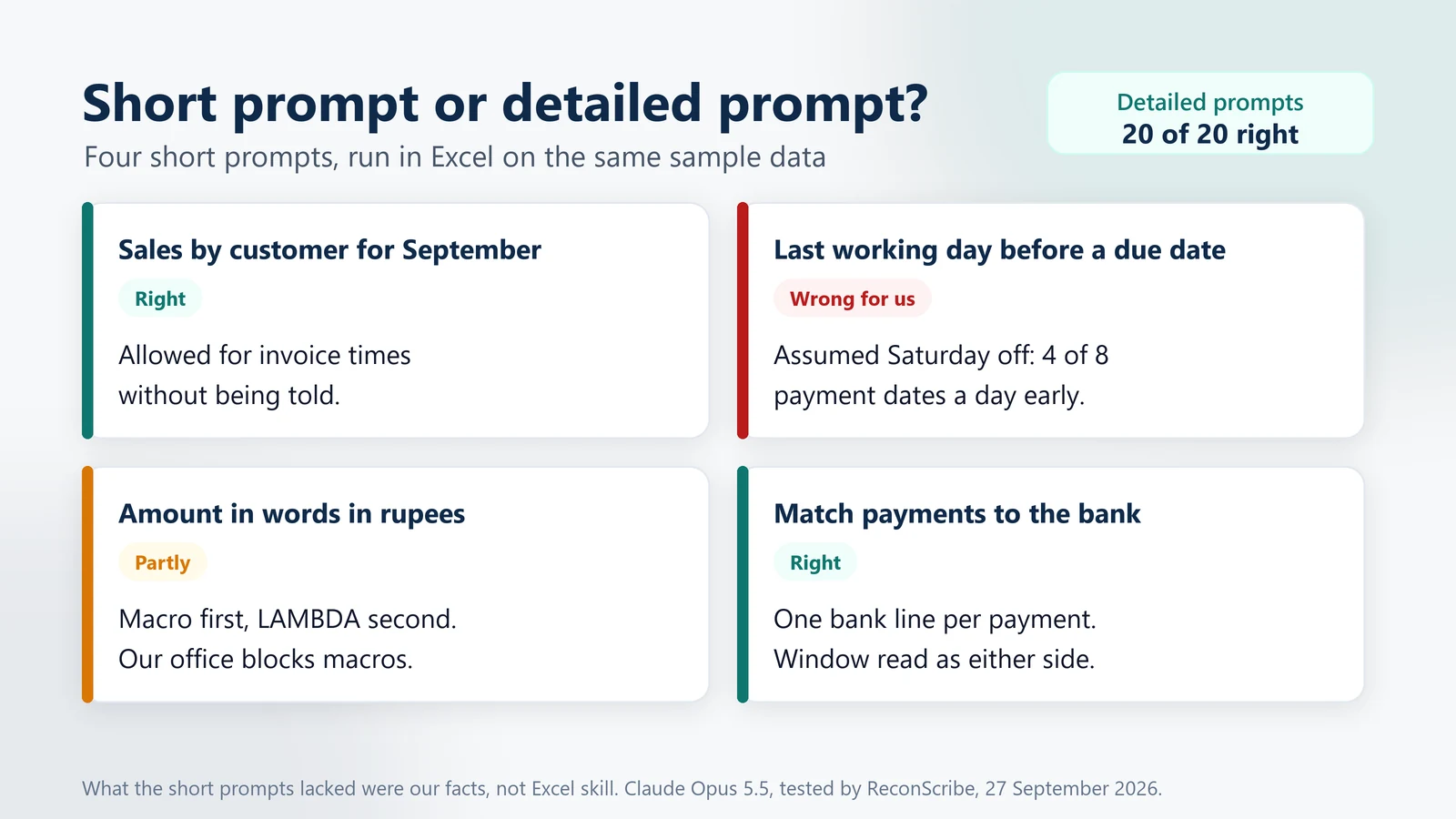
A perfect score says as much about the prompts as about the model, so we ran a side test. We typed four short AI prompts for Excel the way most people do, with no layout, version or house rules, each in a fresh session, and ran the answers against the same data.
| Short prompt | Result | What happened in Excel |
|---|---|---|
| “Total each customer’s sales for September 2026” | Right | Right on our data. It ended the window before 1 October without being told, so the evening invoices were kept. It assumed its own sheet and column letters. |
| “Last working day on or before a due date, skipping holidays” | Wrong for us | Wrong for our office. Its main formula assumed Saturday and Sunday off, so 4 of our 8 payment dates came out a day early. The Monday-to-Saturday version was only a footnote. |
| “Show an amount in words in Indian rupees” | Partly | It gave a VBA macro first and a LAMBDA second. Both are sound, but with macros blocked only the second works; the detailed prompt went straight to it. |
| “Match each payment in my books to the bank: same amount, within 3 days” | Right | Right on our data, one bank line per payment. It read “within 3 days” as either side of the payment date, a fair reading of a vague rule. |
The Excel was never the problem. Even the short prompts produced working formulas, and one of them allowed for invoice times without being told. What a short prompt cannot supply are your facts: that your office works on Saturdays, that macros are blocked, and where your data sits. The payment-date answer is the one to remember. It looked right, ran without an error, and scheduled four of our eight payments a day early.
Eight Excel traps, and what the wrong formula returned
These are the mistakes the traps were built to catch. The AI avoided every one of them in the detailed prompts. The right-hand column is what the common wrong version returned when we ran it in Excel on the same data, so you can see what each mistake costs.
| Trap | The common wrong formula | What it returned in Excel |
|---|---|---|
| Invoices on the last day of the month carry a time | =SUMIFS(... ,"<="&EOMONTH(B1,0)) |
Crest Stationers: ₹81,200 instead of ₹2,05,800. Two evening invoices worth ₹1,82,600 dropped out. |
| The office works on Saturdays | =WORKDAY(E2+1,-1,holidays) |
A Saturday deadline, 16 May 2026, moved back to Friday. |
| Two payments of ₹25,000 on the same day | XLOOKUP on amount and date window only |
Both payments matched the same bank line. |
| Paise in an amount in words | =INT((A2-INT(A2))*100) |
88 paise for ₹12,34,567.89, instead of 89. |
| Excel 2019 array formula entered once over a block | Ctrl+Shift+Enter on F2:F101 at once |
Every cell showed the first vendor. |
| VLOOKUP without its fourth argument on an unsorted list | =VLOOKUP(A2,Vendors!$A$2:$B$8,2) |
7 of 10 vendor names wrong, with no error shown. |
| NPV with the year-0 cost inside the function | =NPV(12%,B3:G3) |
₹34,123 instead of ₹38,218. |
| A band written with < instead of <= | IF(D2-C2<60, ... ) |
₹3,000 late charge at exactly 60 days, instead of ₹2,000. |
Keep company data safe when you use AI with Excel
Spreadsheets carry customer names, bank accounts, PAN and GSTINs. A few habits keep you on the right side of your clients and of the Digital Personal Data Protection Act, 2023:
- Paste sample rows, not the ledger. Twenty rows with the awkward cases are enough to get the formula right. Replace names, PAN, GSTINs and account numbers with codes; every one of these AI prompts for Excel works just as well with codes.
- Know what in-Excel add-ins can read. Copilot in Excel and Claude for Excel can see the open workbook. Keep other sheets and files out of it when you ask for help.
- Test on a copy. Run a new formula or query on a copy of the file and compare a few results with figures you know before it goes into the real workbook.
- Use a business plan with training switched off. The business plans of the main AI tools say they do not train on your chats by default. Check the current terms of the tool you use.
Please note: we update this page from time to time, but Excel, AI tools and tax rules change and there can be a gap between a change and our update. Check any rate or due date on the official portal before you rely on a formula that uses it. These AI prompts for Excel and the tested answers help you work faster; they are not professional advice, and ReconScribe is not responsible for decisions made on them.
Frequently asked questions
What are the best AI prompts for Excel?
The ones that tell the AI your Excel version, where the data sits, which columns are text or numbers, the business rule, and the result you expect. In our test all 20 prompts built that way gave formulas that worked in Excel first time, from SUMIFS and XLOOKUP to Power Query and a LAMBDA.
Do these work as ChatGPT prompts for Excel, or only as Claude AI prompts for Excel?
Yes. They are plain text, so they work in ChatGPT, Gemini, Copilot or Claude, and in add-ins such as Copilot in Excel or Claude for Excel that can read your workbook directly. We tested them in Claude Opus 5.5; other tools can differ, so keep the step where you run the formula on a copy and check the result against a figure you know.
How do I write an AI prompt for an Excel formula?
Name the Excel version, the sheet and range, the header row, and whether each column holds text, numbers or dates. Paste a few sample rows, state the rule, ask for one formula for row 2 to copy down, and ask for the results you should see. The expected results are what let you check it in a minute.
Can AI build an Excel dashboard?
It can plan one and write every KPI formula. In our test it chose the KPIs, the charts and the layout, and found the story in the data: one low-margin order behind a 34% jump in sales. You still build the charts, and on Excel 2021 or 2019 you should say so, or you may get GROUPBY and PIVOTBY formulas that do not exist there.
Which Excel version should I tell the AI?
The one you use: File, Account, About Excel shows it. Excel 2019 has no dynamic arrays; Excel 2021 added XLOOKUP, LET and FILTER; Excel 2024 added LAMBDA and TEXTSPLIT; newer functions such as GROUPBY and the REGEX functions exist only in some Microsoft 365 builds.
Can I trust AI Excel formulas without checking?
No. Our 20 detailed prompts all worked, but in a side test a short prompt for payment dates assumed Saturday was a holiday and moved four of eight dates a day early. Run the formula on a copy of your file and compare a few results with figures you have worked out yourself.
Can AI write Power Query or macros for Excel?
Yes. Its Power Query in our test ran as written and handled a bank file with junk rows, day-first dates and leading zeros. If macros are blocked in your office, say so: it then gives formula or LAMBDA answers, like the amount in words prompt above.
Is it safe to paste company data into an AI tool for Excel help?
Paste sample rows, not the whole ledger, and replace names, PAN, GSTIN and bank account numbers with codes. The formula works the same on sample data. Use a business plan that does not train on your chats, and remember that in-Excel add-ins can read every sheet in the open workbook.
Sources
We checked the answers to these AI prompts for Excel against these official pages on 27 September 2026, and ran every formula in Excel for Microsoft 365.
- What's new in Excel 2021 for Windows and What's new in Excel 2024 (Microsoft Support), for which functions each version has.
- SUMIFS, XLOOKUP, WORKDAY.INTL and LAMBDA function references (Microsoft Support).
- Income-tax Act, 2025, as amended by the Finance Act, 2026, sections 156 and 202, for the new-regime slabs, rebate and marginal relief (Income Tax Department).
- Micro, Small and Medium Enterprises Development Act, 2006, section 15, for the 45-day payment limit (India Code).
- Digital Personal Data Protection Act, 2023 (Ministry of Electronics and Information Technology).
Related guides and tools: AI prompts for accounting, AI prompts for finance, Excel formulas for finance, Excel financial dashboard template, GSTR-2B reconciliation template, income tax slab rates and the EMI loan calculator.