
To use XLOOKUP with multiple criteria, multiply one TRUE or FALSE test per column and look up 1:
=XLOOKUP(1,(criteria_range1=value1)*(criteria_range2=value2),return_range)The three patterns, on the practice file’s own ranges:
=XLOOKUP(1,($B$6:$B$17=K8)*($C$6:$C$17=L8),$G$6:$G$17)=XLOOKUP(1,($C$6:$C$17="Black")+($C$6:$C$17="Navy"),$F$6:$F$17)=XLOOKUP(K7&"|"&L7,$B$6:$B$17&"|"&$C$6:$C$17,$G$6:$G$17)- AND, multiply with *: store in column B, order number in C, amount in G (lesson 2). For EU and 1002 it returns 45.90.
- OR, add with +: color in column C, price in F (lesson 3). It returns the price on the first row that is black or navy. Adding works here because one cell cannot hold both colors.
- Join with & and a
"|"separator: UK and 1003 become the keyUK|1003, which returns 96.00. The separator keeps pairs such asTS|XLandTSX|Lapart.
In Google Sheets, wrap the multiply and join formulas in ARRAYFORMULA, as shown further down.
In the practice file, order 1003 exists in the US, UK and EU stores. A plain XLOOKUP on the order number stops at the first 1003 and returns 210.50 from the US store. With the store as a second test, the formula returns the UK amount, 96.00.
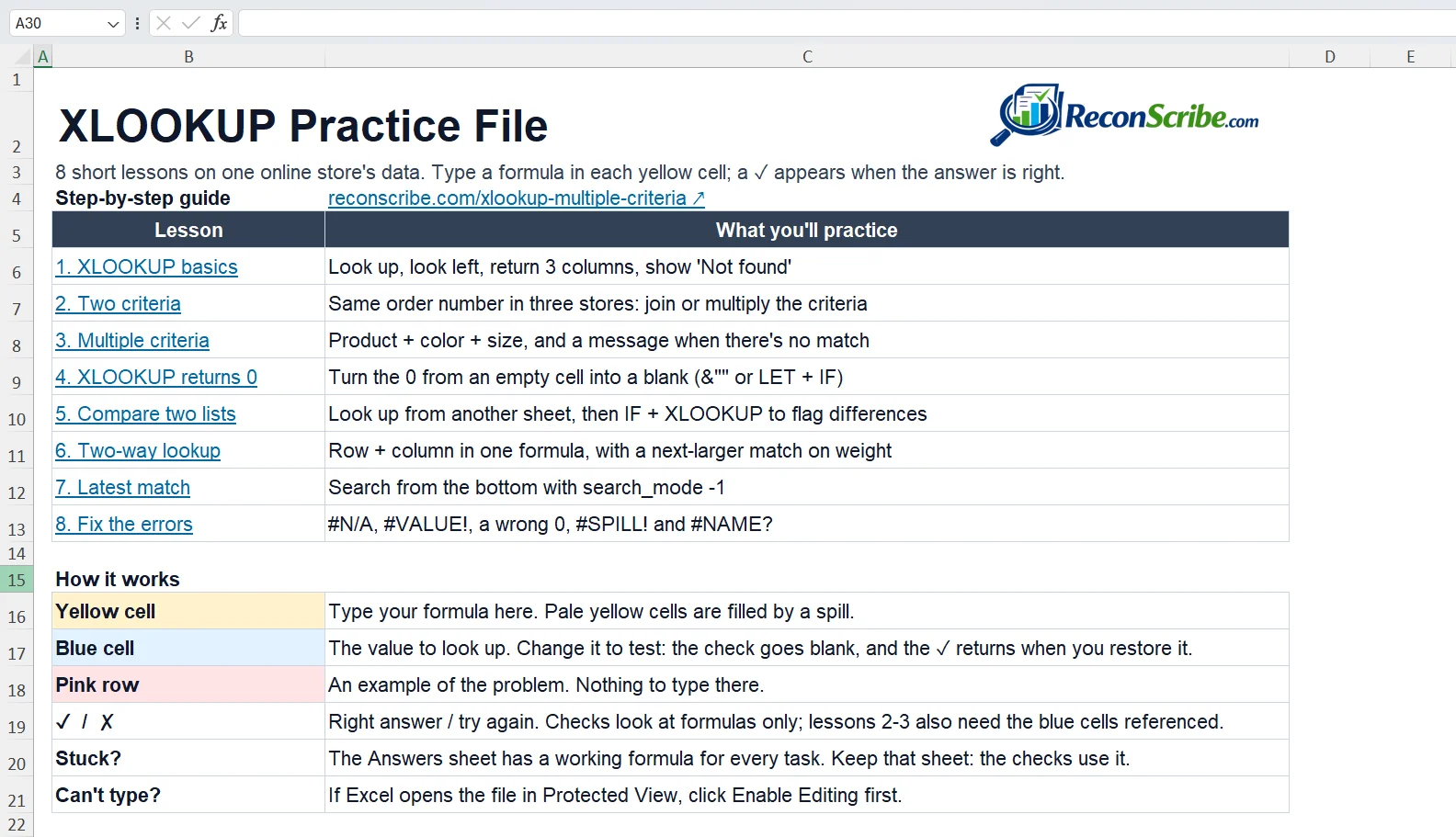
Below are 8 worked examples on the same made-up store: the basics, two and three criteria, a blank instead of 0, two lists on two sheets, a two-way lookup, the latest match and six common errors. Each one is a lesson in a free practice file that shows a ✓ as soon as your answer is right.
Download the free XLOOKUP practice file (Excel, 8 lessons)
Every lesson uses one made-up online store that sells in the US, UK and EU, with the data on the left of each sheet and the tasks on the right. Every example on this page uses this file’s data.
It is a plain .xlsx workbook with formulas only and no macros, last updated 2 November 2026. Open the Start here sheet first, and click Enable Editing if Excel opens the file in Protected View. The sheets are protected except for the cells the lessons use, so try the extra examples on this page in a new workbook.
Watch the XLOOKUP walkthrough
The walkthrough opens with the VLOOKUP trap (insert a column and VLOOKUP quietly returns the wrong column), explains what XLOOKUP is and where VLOOKUP fails, then works through all eight lessons in order, building or fixing each formula and showing the ✓ it earns.
- 0:00 Why XLOOKUP beats VLOOKUP
- 0:20 Start here: the free practice file
- 0:39 What is XLOOKUP?
- 1:11 Where VLOOKUP fails
- 2:43 XLOOKUP basics: look left, 3 columns, not found
- 3:59 XLOOKUP with two criteria: join or multiply
- 5:22 XLOOKUP multiple criteria: product, color, size
- 6:43 XLOOKUP returns 0? Show a blank
- 7:37 Compare two lists on two sheets
- 8:26 Two-way lookup: row and column
- 9:02 Find the latest match
- 10:02 Fix 6 common XLOOKUP errors
- 11:00 Practice file with answers
XLOOKUP syntax: the 6 arguments
XLOOKUP finds a value in one column or row and returns the matching item from another, stopping at the first match. Three arguments are required and three are optional:
=XLOOKUP(lookup_value, lookup_array, return_array, [if_not_found], [match_mode], [search_mode])| Argument | What it does | If you leave it out |
|---|---|---|
| lookup_value | The value to find, such as a SKU. | Required |
| lookup_array | The column or row to search. | Required |
| return_array | What to return, with as many rows as lookup_array (or columns, for a row). | Required |
| if_not_found | What to show when nothing matches. | #N/A |
| match_mode | 0 exact, -1 exact or next smaller, 1 exact or next larger, 2 wildcards. | 0, exact |
| search_mode | 1 first to last, -1 last to first, 2 and -2 binary search on sorted data. | 1, first to last |
Coming from VLOOKUP? XLOOKUP needs no column number, matches exactly by default and can look to the left. Our VLOOKUP, XLOOKUP and INDEX MATCH comparison covers the rest.
XLOOKUP basics: four formulas to start with
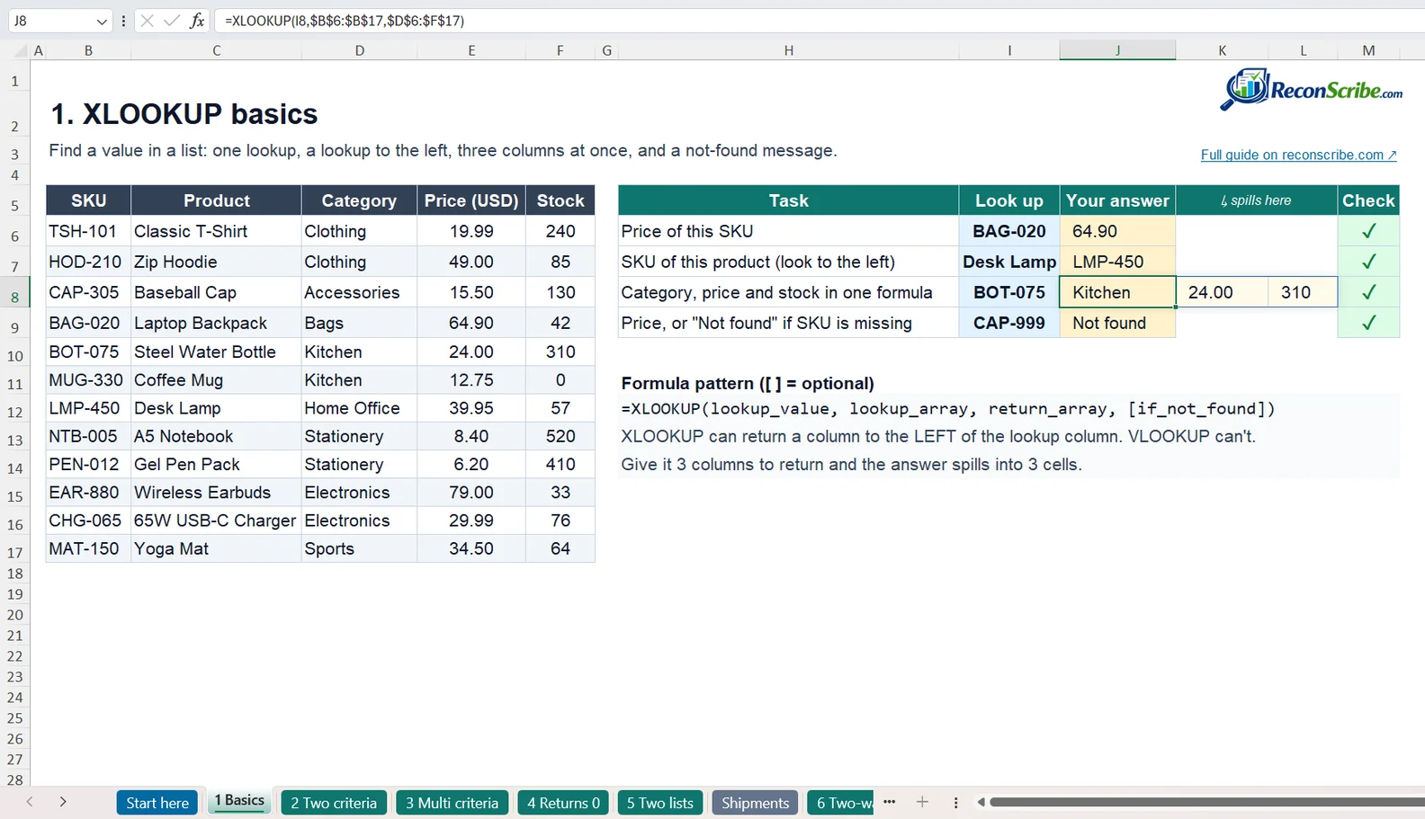
Lesson 1 has 12 products with a SKU (product code), name, category, price and stock in columns B to F. Type these four formulas in J6 to J9:
=XLOOKUP(I6,$B$6:$B$17,$E$6:$E$17)=XLOOKUP(I7,$C$6:$C$17,$B$6:$B$17)=XLOOKUP(I8,$B$6:$B$17,$D$6:$F$17)=XLOOKUP(I9,$B$6:$B$17,$E$6:$E$17,"Not found")- Price by SKU: BAG-020 returns 64.90.
- Look to the left: Desk Lamp returns LMP-450 from column B, left of the product column, which VLOOKUP cannot do.
- Several columns: a three-column return range makes BOT-075 spill Kitchen, 24.00 and 310 into three cells, so keep the two cells to the right empty.
- Your own message: CAP-999 is missing, so the fourth argument shows “Not found” instead of #N/A.
The $ signs lock each range, so the ranges stay in place when you copy the formula down. Without them, the ranges move down as you copy, and the top rows drop out of the search.
XLOOKUP with 2 criteria: join or multiply
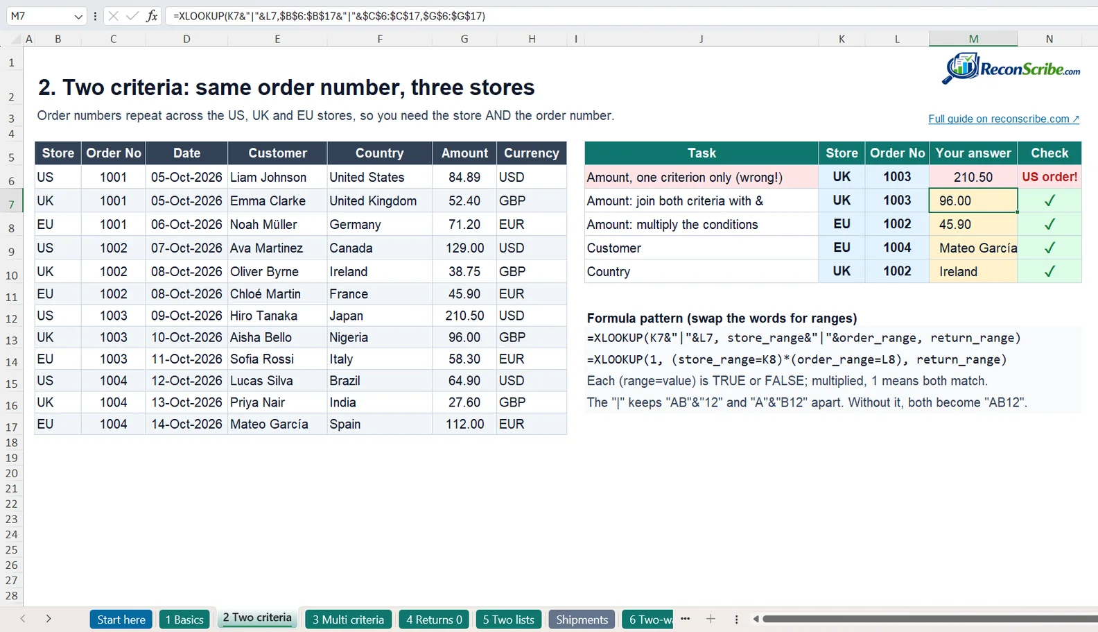
Lesson 2 lists 12 orders from three stores. Each store numbers its own orders, so order 1003 appears three times. Look up the UK order by number alone and XLOOKUP stops at the first 1003:
=XLOOKUP(L6,$C$6:$C$17,$G$6:$G$17)That returns 210.50 from the US store instead of the UK amount, 96.00, and nothing warns you. There are two ways to match both the store and the order number.
Method 1: join the criteria with & and a separator
Join the two values into one key, and the two columns the same way, so UK|1003 is compared with US|1001, UK|1001 and so on down the list:
=XLOOKUP(K7&"|"&L7,$B$6:$B$17&"|"&$C$6:$C$17,$G$6:$G$17)It returns 96.00. Keep the "|" separator: without it, different pairs can produce the same key. Product TS in size XL and product TSX in size L both become TSXL, and XLOOKUP returns whichever comes first. With it they stay TS|XL and TSX|L. Use a character that never appears in your data.
Method 2: multiply the conditions and look up 1
Write one test per criterion in parentheses, multiply them, and look up 1:
=XLOOKUP(1,($B$6:$B$17=K8)*($C$6:$C$17=L8),$G$6:$G$17)Each test returns 12 TRUE or FALSE values. Multiplying turns TRUE into 1 and FALSE into 0, so a row scores 1 only when both tests are true (TRUE*TRUE=1). For EU and 1002 the result is {0;0;0;0;0;1;0;0;0;0;0;0}, so XLOOKUP finds the single 1 and returns 45.90. Change the return range to get another column:
| Task | Store | Order No | Result |
|---|---|---|---|
| Amount, order number only (wrong) | UK | 1003 | 210.50, the US order |
| Amount, join method | UK | 1003 | 96.00 |
| Amount, multiply method | EU | 1002 | 45.90 |
| Customer, multiply method | EU | 1004 | Mateo García |
| Country, join method | UK | 1002 | Ireland |
Which one to use: for XLOOKUP with 2 criteria and exact matches, the join is easier to read. Multiplying works better for three or more criteria and accepts any test, such as ($G$6:$G$17>50) for amounts over 50. On very large tables, a helper column that joins the criteria once can be faster.
XLOOKUP with multiple criteria (3 or more)
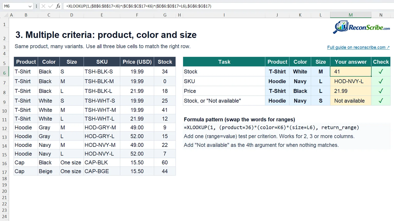
Lesson 3 lists 12 variants of a T-shirt, a hoodie and a cap by color and size, each with a SKU, price and stock. A lookup on the product alone returns the first T-shirt row, black in small at 19.99, when you want black in large at 21.99. Add one test per column:
=XLOOKUP(1,($B$6:$B$17=J8)*($C$6:$C$17=K8)*($D$6:$D$17=L8),$F$6:$F$17)Only the T-Shirt, Black, L row multiplies to 1, so the formula returns 21.99. Each extra criterion is one more test and one more *. To return another column, change only the return range:
| Task | Product | Color | Size | Result |
|---|---|---|---|---|
| Stock | T-Shirt | White | M | 41 |
| SKU | Hoodie | Navy | L | HOD-NVY-L |
| Price | T-Shirt | Black | L | 21.99 |
| Stock, or a message | Hoodie | Navy | S | Not available |
There is no navy hoodie in small, so the last task adds a message as the fourth argument:
=XLOOKUP(1,($B$6:$B$17=J9)*($C$6:$C$17=K9)*($D$6:$D$17=L9),$G$6:$G$17,"Not available")XLOOKUP multiple results: use FILTER instead
XLOOKUP returns one match. To list every match, give the same tests to FILTER. This one lists the black T-shirt sizes in stock, with a greater-than test on the stock column:
=FILTER($D$6:$D$17,($B$6:$B$17="T-Shirt")*($C$6:$C$17="Black")*($G$6:$G$17>0))It spills S and L, since the medium has 0 in stock. For OR logic, add tests instead of multiplying them: ($C$6:$C$17="Black")+($C$6:$C$17="Navy") keeps either color.
XLOOKUP multiple criteria in Google Sheets
Google Sheets has XLOOKUP too, and the multiply method works there once you wrap it in ARRAYFORMULA. Press Ctrl+Shift+Enter (Cmd+Shift+Enter on a Mac) while you edit the formula, and Sheets adds the wrapper for you:
=ARRAYFORMULA(XLOOKUP(1,(B6:B17=J8)*(C6:C17=K8)*(D6:D17=L8),F6:F17))The join method needs the same wrapper. The practice file is made and tested for Excel, so practice there and copy the pattern to Sheets.
XLOOKUP returns 0? Show a blank instead
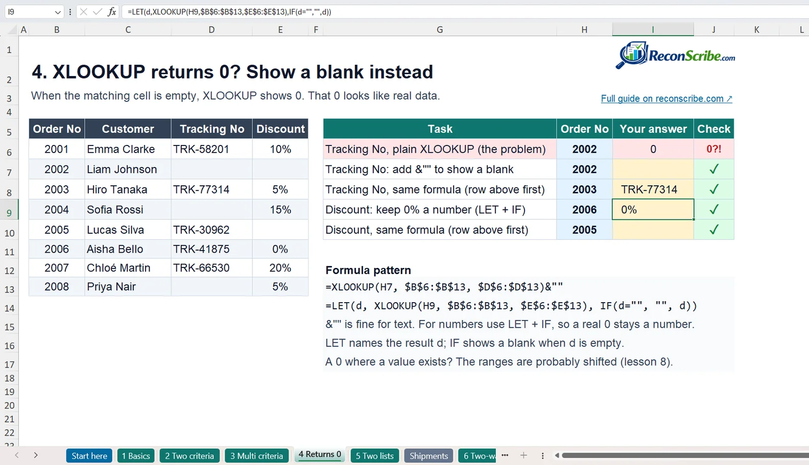
Lesson 4 lists 8 orders, and some tracking numbers and discounts are still empty. Order 2002 has no tracking number yet, but a plain XLOOKUP shows 0:
=XLOOKUP(H6,$B$6:$B$13,$D$6:$D$13)The lookup worked: it returned the order’s tracking cell, which is empty, and a formula that returns an empty cell shows 0, just as =D7 does when D7 is empty. That is why if_not_found does not help here. There are two fixes.
For text: add an empty string
=XLOOKUP(H7,$B$6:$B$13,$D$6:$D$13)&""Joining "" turns the result into text, so the empty cell shows as a blank while order 2003 still shows TRK-77314. Use it for text such as tracking numbers or notes.
For numbers and dates: LET and IF
=LET(d,XLOOKUP(H9,$B$6:$B$13,$E$6:$E$13),IF(d="","",d))LET names the result d, so the lookup runs once, and IF shows a blank only when d is empty. Order 2006 keeps its real 0% discount as a number, and order 2005, with no discount, shows a blank. With &"" instead, that 0% would become the text “0”, which SUM and AVERAGE skip.
XLOOKUP returns 0 but the value exists?
Check these four causes in order:
- The return cell is empty. It shows as 0, or as a date such as 1/0/1900 or 00-Jan-1900 in a date column. Use one of the two fixes above.
- The ranges do not line up. If the return range starts a row lower than the lookup range, every answer comes from the next row, as lesson 8 shows. Start both ranges on the same row.
- The value is in the list twice. XLOOKUP stops at the first match, as with order 1003 in lesson 2, and that row may hold the empty cell. Add a second criterion.
- The 0 is your own. In lesson 5, if_not_found is 0, so a 0 means the order is not on the Shipments sheet.
The number format 0;-0;;@ hides zeros on screen, but it hides real zeros too, and it rounds 21.99 to 22. For prices, use #,##0.00;-#,##0.00;;@ instead.
XLOOKUP from another sheet: compare two lists
Lesson 5 checks 8 orders against a Shipments sheet that lists only 6 of them, in a different order. This formula returns each shipped quantity, or 0 for orders that are not on that sheet:
=XLOOKUP(B6,Shipments!$B$5:$B$10,Shipments!$D$5:$D$10,0)Click the Shipments tab while you type to pick its ranges. Excel adds the sheet name and an exclamation mark, plus single quotes if the name has a space, as in 'Shipments 2026'!$B$5:$B$10. Press F4 (Fn+F4 on some laptops, Cmd+T on a Mac) to lock the ranges, fill down, then compare the two quantities in column F:
=IF(E6=D6,"OK",IF(E6=0,"Not shipped","Short"))| Order No | Qty ordered | Qty shipped | Status |
|---|---|---|---|
| 3001 | 2 | 2 | OK |
| 3002 | 5 | 3 | Short |
| 3003 | 1 | 1 | OK |
| 3004 | 3 | 0 | Not shipped |
| 3005 | 4 | 4 | OK |
| 3006 | 2 | 1 | Short |
| 3007 | 6 | 0 | Not shipped |
| 3008 | 1 | 1 | OK |
Two orders are short and two have not shipped. You can also look up all 8 order numbers at once. With E7:E13 empty, type this in E6, and the results spill down to E13:
=XLOOKUP(B6:B13,Shipments!$B$5:$B$10,Shipments!$D$5:$D$10,0)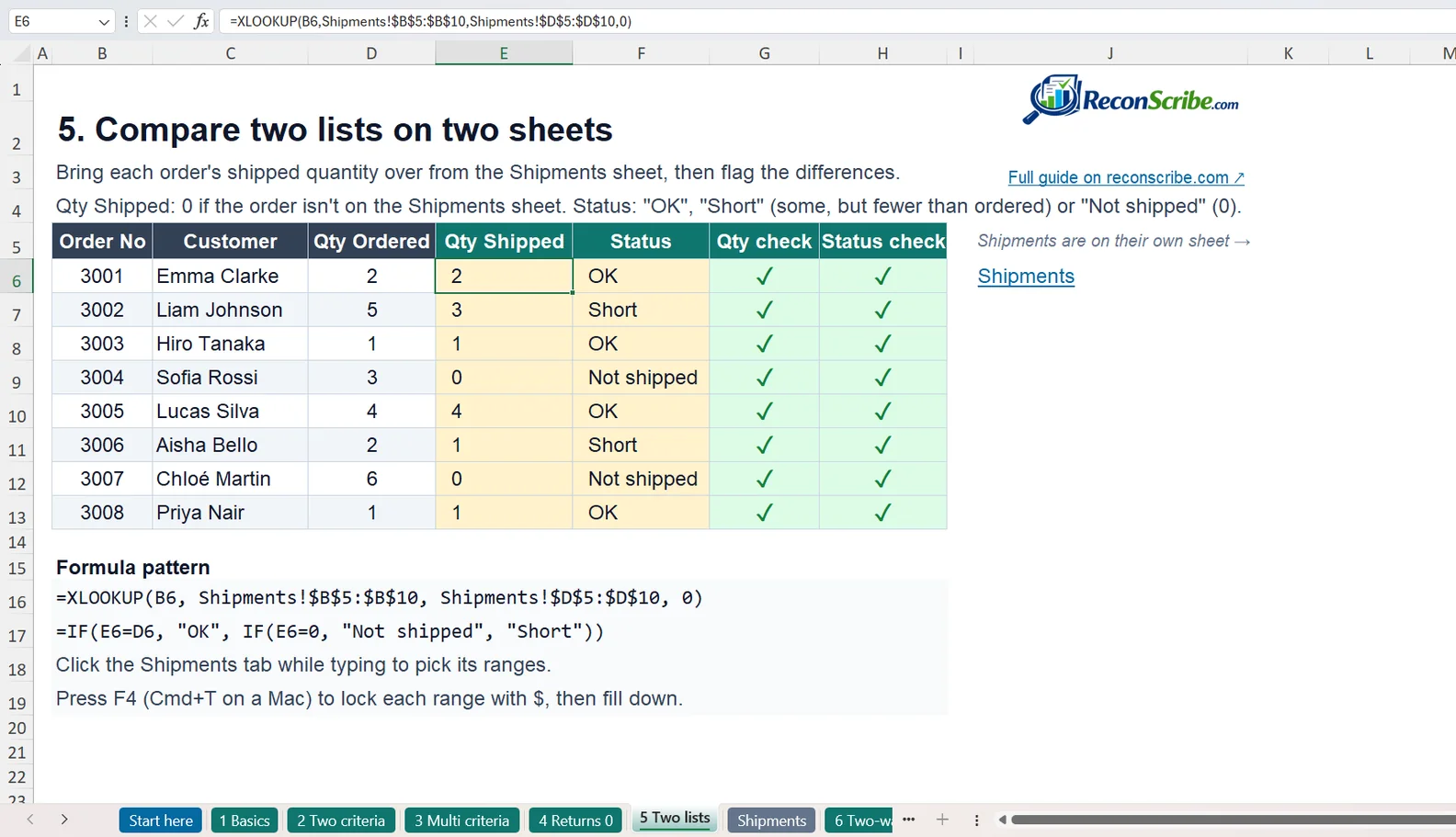
Two-way XLOOKUP: criteria in rows and columns
Lesson 6 prices parcels from a rate table with four zones down the side and five weight bands across the top. Each band is an upper limit, so a 1.4 kg parcel falls in the band up to 2 kg:
| Zone | Up to 0.5 kg | Up to 1 kg | Up to 2 kg | Up to 5 kg | Up to 10 kg |
|---|---|---|---|---|---|
| Zone 1 | 4.50 | 5.90 | 7.80 | 11.50 | 16.00 |
| Zone 2 | 8.90 | 10.50 | 13.20 | 19.90 | 28.00 |
| Zone 3 | 14.00 | 17.50 | 22.00 | 33.00 | 47.50 |
| Zone 4 | 19.50 | 24.00 | 31.00 | 46.00 | 66.00 |
One XLOOKUP inside another finds the column, then the row:
=XLOOKUP(J6,$B$6:$B$9,XLOOKUP(K6,$C$5:$G$5,$C$6:$G$9,,1))The inner XLOOKUP uses match_mode 1, exact or next larger, to pick the weight band and return its column of four rates. The outer one picks the zone from that column, so zone 2 at 0.3 kg returns 8.90, zone 3 at 1.4 kg returns 22.00, zone 1 at 4.2 kg returns 11.50 and zone 4 at 7.5 kg returns 66.00.
Without match_mode, 1.4 kg returns #N/A, because 1.4 is not in the header row. With -1 it returns 17.50, the 1 kg rate, which undercharges. Use -1 when each limit is a starting point, such as a discount that starts at 10 units.
The inner XLOOKUP is a horizontal lookup: it searches the header row C5:G5, so XLOOKUP replaces HLOOKUP too. When your criteria are in header rows across the top, multiply one test per header row and return a row of the same width:
=XLOOKUP(1,(header_row1=value1)*(header_row2=value2),result_row)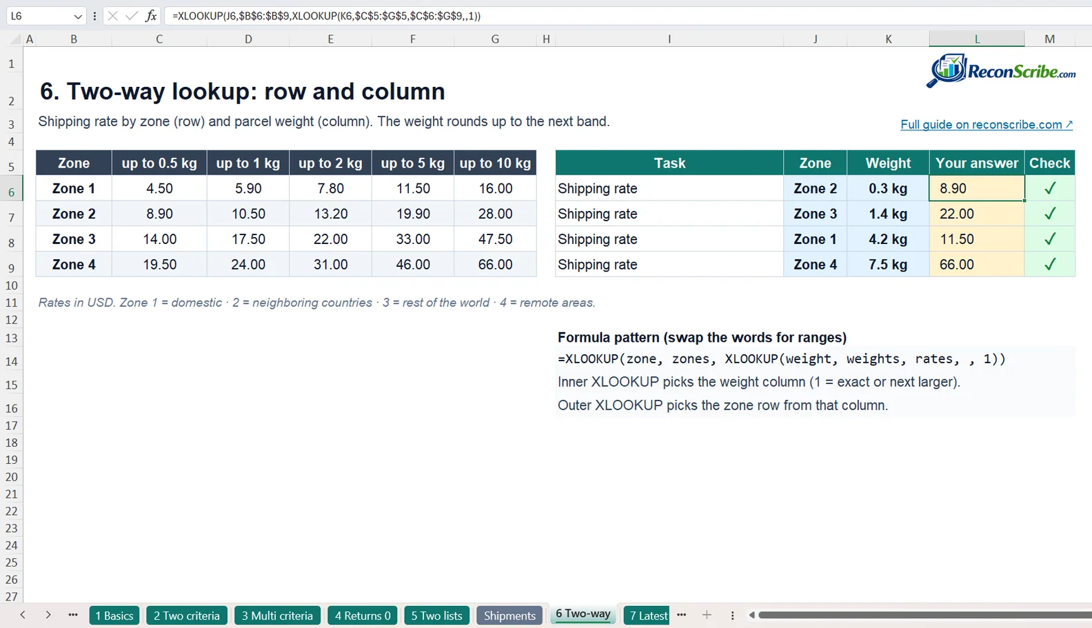
XLOOKUP last match: find the latest order
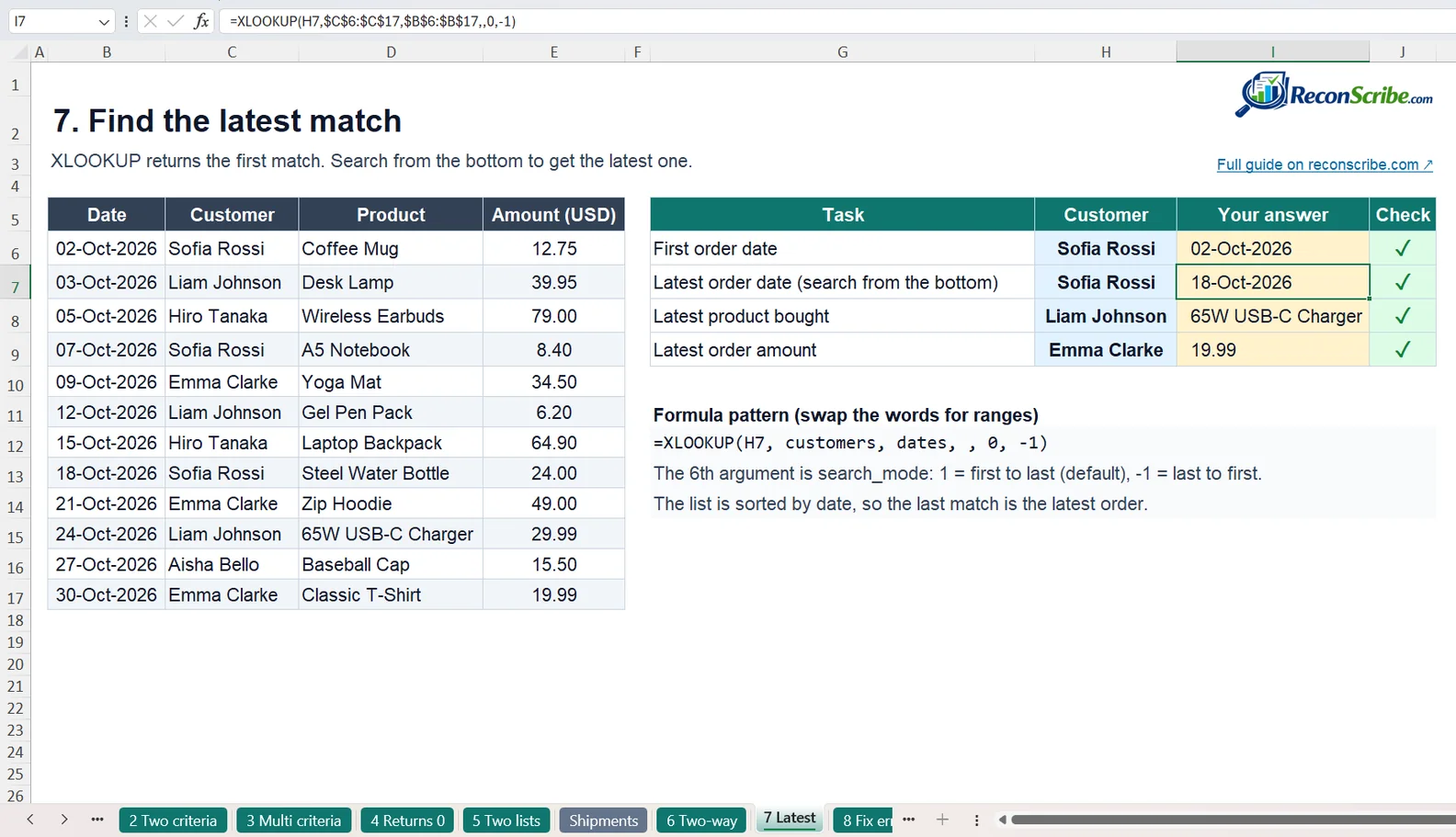
Lesson 7 is an order log of 12 rows in date order, and some customers appear more than once. XLOOKUP returns the first match, so a lookup on Sofia Rossi returns her oldest order date, 2 October 2026. Set the sixth argument, search_mode, to -1 and it searches from the bottom up:
=XLOOKUP(H7,$C$6:$C$17,$B$6:$B$17,,0,-1)Now it returns 18 October 2026, her latest order. The empty argument between the commas skips if_not_found, and 0 keeps the exact match. On the product column, Liam Johnson’s latest purchase is the 65W USB-C Charger; on the amount column, Emma Clarke’s latest order is 19.99.
Sort the list first. A reverse search returns the last match in the list, which is the latest only when rows run from oldest to newest. If yours do not, find the latest date with MAXIFS and use it as a second criterion:
=XLOOKUP(1,($C$6:$C$17=H8)*($B$6:$B$17=MAXIFS($B$6:$B$17,$C$6:$C$17,H8)),$D$6:$D$17)On the practice data it also returns the 65W USB-C Charger, and it works even when the rows are not sorted. Type it in I8 and it earns the same ✓.
XLOOKUP not working? 6 errors and fixes
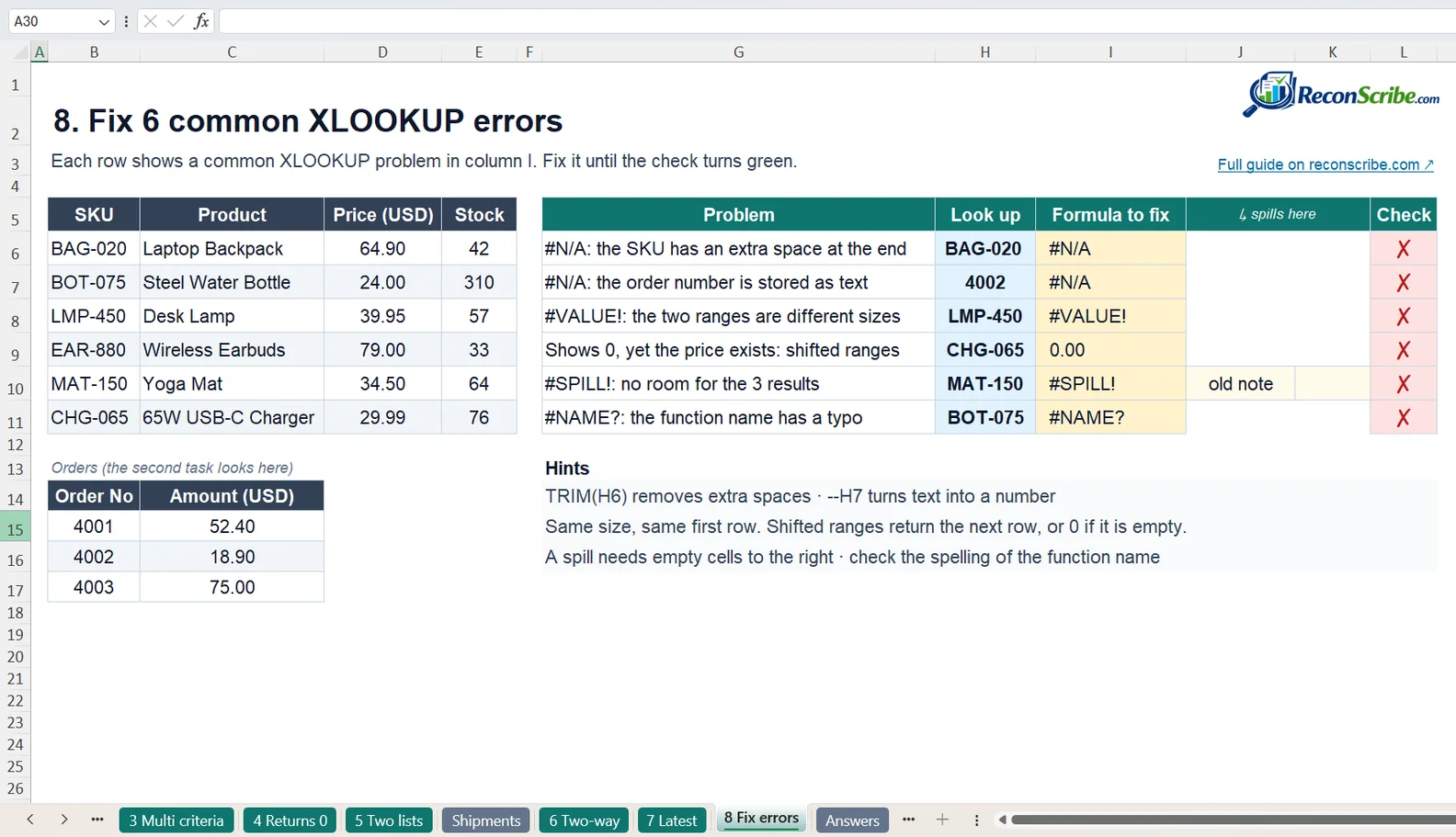
Lesson 8 opens with six broken formulas, each a common XLOOKUP problem. Each fix turns a ✗ into a ✓:
| Error | Cause in the practice file | Fix | Result |
|---|---|---|---|
| #N/A | The SKU BAG-020 has a space at the end. | Wrap it in TRIM(H6). |
64.90 |
| #N/A | Order 4002 is stored as text, and the list holds numbers. | Convert it with --H7 (two minus signs turn text into a number). |
18.90 |
| #VALUE! | The lookup range has 6 rows and the return range 5. | Make the ranges the same size. | 39.95 |
| A wrong 0 | The return range starts a row lower, so CHG-065 lands on an empty cell. | Start both ranges on the same row. | 29.99 |
| #SPILL! | An old note in J10 blocks the 3 results. | Clear the cell in the way. | Yoga Mat, 34.50, 64 |
| #NAME? | XLOOKUP is spelled XLOKUP. | Fix the spelling. | 310 |
Shifted ranges are the risky one. They show 0 here only because the row under the list is empty. For other SKUs they return the next row’s value with no error at all: BAG-020 gets 24.00, the price of the bottle below it.
If the space or the text is in the list instead, clean the range inside the formula, as in =XLOOKUP(TRIM(H6),TRIM($B$6:$B$11),$D$6:$D$11), or look up H7&"" when the list holds numbers stored as text.
Do not hide errors with IFERROR. It swaps the error for a 0 or a blank that looks like a real answer, and the practice file’s checks reject it. Fix the cause, and keep if_not_found for values that are truly missing.
#NAME? with XLOOKUP spelled right usually means your Excel has no XLOOKUP. Excel 2019 and older show it as _xlfn.XLOOKUP in files made in newer versions. Text typed without quotes, such as Not found in the fourth argument, gives the same error.
What is inside the practice file
| Sheet | What it does | Do you type here? |
|---|---|---|
| Start here | Links to each lesson, the color key and the Excel versions you need. | No |
| 1 Basics | Price by SKU, a lookup to the left, three columns at once, a not-found message. | Yellow cells only |
| 2 Two criteria | One order number in three stores. | Yellow cells only |
| 3 Multi criteria | Product, color and size in one lookup. | Yellow cells only |
| 4 Returns 0 | A blank instead of 0 for empty cells. | Yellow cells only |
| 5 Two lists | Orders checked against shipments on another sheet. | Yellow cells only |
| Shipments | The second list for lesson 5. | No |
| 6 Two-way | Shipping rate by zone and weight. | Yellow cells only |
| 7 Latest | First and latest order for a customer. | Yellow cells only |
| 8 Fix errors | Six broken formulas to repair. | Yellow cells, plus clear J10 |
| Answers | A working formula and the expected result for every task. The checks read it. | No |
The colors mean the same thing on every lesson sheet, and Start here has the key:
- Yellow cells: type your formula here.
- Blue cells: the values to look up. Change one to test your formula: its ✓ or ✗ disappears, and comes back when you change the value back.
- Pink rows: an example of the problem, in lessons 2 and 4. Nothing to type there.
- ✓ and ✗: ✓ means right, ✗ means try again. In lessons 2 and 3 the formula must also use every blue cell in its row.
Which Excel versions have XLOOKUP (and Google Sheets)
XLOOKUP works in Excel for Microsoft 365 on Windows, Mac, the web and mobile, and in Excel 2021 and Excel 2024. Microsoft says it is not available in Excel 2016 or Excel 2019: those versions open the file, but the formula shows as _xlfn.XLOOKUP and returns #NAME? once it recalculates.
| Excel version | XLOOKUP | LET, FILTER and spilled results |
|---|---|---|
| Excel for Microsoft 365 (Windows, Mac, web) | Yes | Yes |
| Excel 2024 | Yes | Yes |
| Excel 2021 | Yes | Yes |
| Excel 2019, 2016 and older | No, shows #NAME? | No |
Google Sheets has had XLOOKUP since 2022. The arguments work the same way under different names, and the lookup range must be a single row or column. Formulas from this guide that multiply or join ranges need ARRAYFORMULA in Sheets, as shown above. The practice file is built and tested for Excel, so its checks need Excel.
Excel in another language translates the name: XLOOKUP is BUSCARX in Spanish, PROCX in Portuguese (Brazil), XVERWEIS in German, RECHERCHEX in French, CERCA.X in Italian and X.ZOEKEN in Dutch. Japanese Excel keeps the English name, XLOOKUP. Where the comma is the decimal separator, Excel usually expects semicolons between arguments, as in =XLOOKUP(I6;$B$6:$B$17;$E$6:$E$17), or =PROCX(I6;$B$6:$B$17;$E$6:$E$17) in Portuguese. Formulas already in the practice file switch by themselves.
Who this practice file is for
It is for anyone who keeps products, orders, prices or stock in Excel and wants more than a one-column lookup: store and operations staff, analysts, students and self-learners. It needs Excel for Microsoft 365, Excel 2021, Excel 2024 or Excel for the web, so it does not work in Excel 2019 or older, and it is not made for Google Sheets. It does not cover VLOOKUP or INDEX MATCH.
Related guides
- Excel formulas for finance: VLOOKUP vs XLOOKUP, INDEX MATCH and what each Excel error means.
- VLOOKUP in 6 minutes (video): for files that must still open in Excel 2019.
- AI prompts for Excel: 20 tested prompts that write and explain formulas.
- Bank reconciliation template: matching two lists of transactions, a bigger lesson 5.
- Excel financial dashboard template: ten designs on one data table.
- Bank statement to Excel: statement data in clean rows you can look up.
Please note: Excel functions and the versions that include them change, and there can be a gap between a change and our update. Check Microsoft’s documentation for your version before you rely on a formula. This guide and the practice file are for learning, not professional advice, and ReconScribe is not responsible for decisions made on them.
XLOOKUP multiple criteria FAQ
How do you use XLOOKUP with multiple criteria?
Multiply one TRUE or FALSE test per column and look up 1, as in =XLOOKUP(1,(B6:B17=K8)*(C6:C17=L8),G6:G17). Only a row where every test is true multiplies to 1, so XLOOKUP returns that row. Joining the criteria with & and a separator, such as a vertical bar, also works.
Can XLOOKUP return multiple results?
Not from several rows. XLOOKUP returns one match per lookup value: the first, or the last one when search_mode is -1. That row can fill several columns, as in lesson 1, where one formula spills the category, price and stock. To list every row that meets your criteria, use FILTER with the same tests, as in =FILTER(D6:D17,(B6:B17=J6)*(C6:C17=K6)). FILTER needs Excel for Microsoft 365, Excel 2021 or Excel 2024.
Why does XLOOKUP return 0 instead of a blank?
The match was found, but the cell it returns is empty, and a formula that returns an empty cell shows 0. For text, add &"" to the formula. For numbers and dates, use =LET(d,XLOOKUP(...),IF(d="","",d)) so a real 0 stays a number.
Does XLOOKUP with multiple criteria work in Google Sheets?
Yes. Google Sheets has had XLOOKUP since 2022, with the same arguments under different names. Wrap a multiply or join formula in ARRAYFORMULA there, as in =ARRAYFORMULA(XLOOKUP(1,(B6:B17=K8)*(C6:C17=L8),G6:G17)). The practice file is built and tested for Excel, so its self-checks need Excel.
Why does XLOOKUP return #N/A when the value is in the list?
Usually the two values only look the same. A space at the end stops the match, so wrap the lookup value in TRIM. A number stored as text never matches a real number, so convert it with --H7 or VALUE before the lookup.
How do you find the last match with XLOOKUP?
Set the sixth argument, search_mode, to -1 so XLOOKUP searches from the bottom up, as in =XLOOKUP(H7,C6:C17,B6:B17,,0,-1). That is the last match in the list, which is the latest one only when the rows are sorted from oldest to newest.
Which Excel versions have XLOOKUP?
Excel for Microsoft 365 on Windows, Mac, the web and mobile, Excel 2021 and Excel 2024. Excel 2019, Excel 2016 and older do not have it, and formulas that use it return #NAME? there. LET, FILTER and spilled results need the same versions.
Sources
- Microsoft Support, XLOOKUP function
- Microsoft Support, LET function
- Microsoft Support, Excel functions (alphabetical)
- Microsoft Support, Dynamic array formulas and spilled array behavior
- Microsoft Support, How to correct a #SPILL! error
- Microsoft Support, How to correct a #NAME? error
- Microsoft Support, Display or hide zero values
- Google Docs Editors Help, XLOOKUP function
- Google Workspace Updates, Adding more flexibility to functions in Sheets